clear all syms f(x1,x2) gradf(x1,x2) Hf(x1,x2); f(x1,x2) = -log(1-x1-x2)-log(x1)-log(x2); gradf(x1,x2)=gradient(f); Hf(x1,x2)=hessian(f); N=30;%number of Newton iterations tol=0.00001; x=zeros(2,N); fval=zeros(N,1); er=zeros(N,1); x(:,1)=[.8;.1];%initial point k=1;while norm(double(gradf(x(1,k),x(2,k)))) > tol && k < N fval(k) = double(f(x(1,k),x(2,k))); er(k)=norm([1/3;1/3]-x(:,k)); x(:,k+1) = x(:,k) - double(Hf(x(1,k),x(2,k)))\double(gradf(x(1,k),x(2,k))); k=k+1;end fval(k)=double(f(x(1,k),x(2,k))); er(k)=norm([1/3;1/3]-x(:,k)); format long [(1:k)' x(:,1:k)' er(1:k) fval(1:k)]
Press ? for presentation controls.
Best viewed in Firefox,
Chrome and
Opera.
Introduction to
Numerical Analysis
Numerical calculations:
Floating-point systems

We need to represent numbers somehow...
Before even starting to solve any problem numerically, we have to establish one thing:How much information is contained in a number?
Suppose you need to write the actual value of a number, say $\sqrt{2}$, for instance on a piece of paper or on a segment of RAM. The symbol $\sqrt{2}$ obviously is not the value of the number, it just explains to the reader which number we are talking about: is the positive number whose square is equal to 2.Numbers in base 10
What do we mean when we write $647$? As we know since elementary school,Ok, so how about $\sqrt{2}$?!
If one starts evaluating $\sqrt{2}$ in decimal notation, soon suspects the truth:Why is $\sqrt{2}$ irrational?
Now, $\sqrt{2}$ cannot be written as $\frac{m}{n}$ for two integers $m,n$. Indeed, if $$\sqrt{2}=\frac{m}{n}$$ then $$m^2=2n^2$$ but this cannot be: in $m^2$ there is either none or an even number of factors 2, in $2n^2$ there is an odd number of factors 2!Ok. So... how much information is contained in $\sqrt{2}$?
Since the number of digits is infinite and they do not repeat, the decimal expression of $\sqrt{2}$ contains an infinite amount of information. Hence, there is no way to store the value of an irrational number in any physical device. In other words, when we assign, in some computer language, $\sqrt{2}$ to a variable $a$, the value of $a$ is not $\sqrt{2}$ but an approximation of it. In particular, $a^2$ is not exactly equal to 2!What if I just use rational numbers?
The situation does not improve much with decimal rational numbers. On one side, in any base most rational numbers have a periodic pattern after the dot. Since a concrete system can only store a finite number of digits, when we assign such number to a variable, that variable has a slightly different value. The code below shows the effects of this fact:What if I just use rational numbers?
The situation does not improve much with decimal rational numbers. On the other side, given any integer $k$, most rational numbers with a finite number of digits have a number of digits larger than $k$, so even most of these numbers cannot be represented exactly in any given system of numbers representation.What do we learn from here?
In any concrete system of numbers representation, that we did not describe yet, only very few numbers can be represented exaclty:Floating Point = Scientific Notation
Every person that studied some natural science knows how to write a number in scientific notation. For instance,Floating Point Systems
Floating point systems are exactly the convergence of- a base, namely an integer larger than 1;
- an integer $k$, specifying how many digits are kept;
- a range for the exponent.
A toy-model Floating Point Systems in base 10
Here is a simple but instructive example of floating point system. We keep only 3 (decimal) digits and we allow exponents in the range $-10,\dots,10$. Hence,A toy-model Floating Point Systems in base 10
The largest number we can represent in this system isSome interesting calculation
The fact that each number is represented by a fixed number of digits determines a series of important consequences: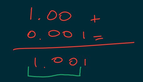
Some interesting calculation
The fact that each number is represented by a fixed number of digits determines a series of important consequences: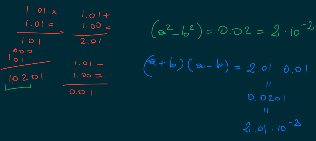
Some interesting calculation
The fact that each number is represented by a fixed number of digits determines a series of important consequences:Recall that, due to round-off, we must always assume
an error of $1$ on the last digit of $a$ and $b$.
Let us evaluate the absolute and relative errors
of the sum and difference of these two numbers:

A common feature
The three problems shown in the three slides above are in fact a common feature of every floating point system and you should always keep them in mind when making your numerical calculations!!Double precision numbers
What is the floating point system used in nowadays computers? Due to technical restrictions (i.e. we can only build miniaturized physical devices with 2 states) modern computers use base 2 to represent numbers. The standard representation for numbers is called double precision for historical reasons. The number of digits allocated for each number is $k=52$ and the exponent ranges from $-1022$ to $1023$.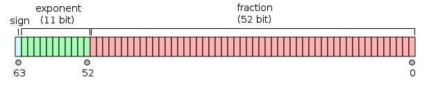
Binary Numbers
Representing numbers in base 2 works exactly as in base 10, with two differences:Examples of binary integers
$1_2 = 1\times2^0 = 1$; $10_2 = 1\times2^1+0 \times2^0 = 2$; $11_2 = 1\times2^1+1 \times2^0 = 3$; $100_2 = 1\times2^2+0\times2^1+0\times2^0 = 4$; $101_2 = 1\times2^2+0\times2^1+1\times2^0 = 5$; $1000_2 = 1\times2^3+0\times2^2+0\times2^1+0\times2^0 = 8$; $1000000_2 = 1\times2^6 = 64$;Examples of fractional binaries
$0.1_2 = 1\times2^{-1} = \frac{1}{2}=0.5$; $0.01_2 = 1\times2^{-2} = \frac{1}{4}=0.25$; $0.11_2 = 1\times2^{-1}+1\times2^{-2} = \frac{3}{4}=0.75$; $0.001_2 = 1\times2^{-3} = \frac{1}{8}=0.125$; $0.0001_2 = 1\times2^{-4} = \frac{1}{16}=0.0625$; $1.1_2 = 1\times2^{0} + 1\times2^{-1} = 1.5$;Largest and smallest number in double precision
Now we are ready to evaluate the largest and smallestpositive numbers representable in double precision. Largest: $1.1\dots1_2\times2^{1023}\simeq2^{1024}\simeq1.8\times10^{308}$ Smallest: $1.0\dots0_2\times2^{-1022}\simeq2\times10^{-308}$
Examples of rationals in binary
- $\frac{1}{2} = 0.1_2$;
- $\frac{1}{3} = 0.01010101\dots_2$;
- $\frac{1}{4} = 0.01_2$;
- $\frac{1}{5} = 0.001100110011\dots_2$;
- $\frac{1}{6} = \frac{1}{3}\times\frac{1}{2}=0.001010101\dots_2$;
- $\frac{1}{7} = 0.001001001\dots_2$;
- $\frac{1}{8} = 0.001_2$;
- $\frac{1}{9} = 0.000111000111\dots_2$;
- $\frac{1}{10} = \frac{1}{5}\times\frac{1}{2} = 0.0001100110011\dots_2$;
Be aware of round-off
From the examples above we see that very few numbers can be represented exactly in double precision: even $0.1$ can be represented only approximatively!! (on the contrary, $0.5$ is represented exactly because $0.5=1/2$)What is numerical analysis
An example: evaluating the derivative of a function.

What is numerical analysis
We already pointed out that numerical computations are subject to errors as soon as a variable is set, due to the fact that almost all numbers write with an infinite number of digits after the dot. Numerical analysis, though, is much more than the study of error propagation in calculation. Following Trefethen, we believe that Numerical Analysis is the study of algorithmsto approximate solutions of problems of continuous mathematics. To keep things concrete, we present below an elementary example of numerical algorithm. This example will also introduce us
to the other main source of errors in NA: the one due to truncation of expressions
involving infinitely many terms or infinitely many steps.
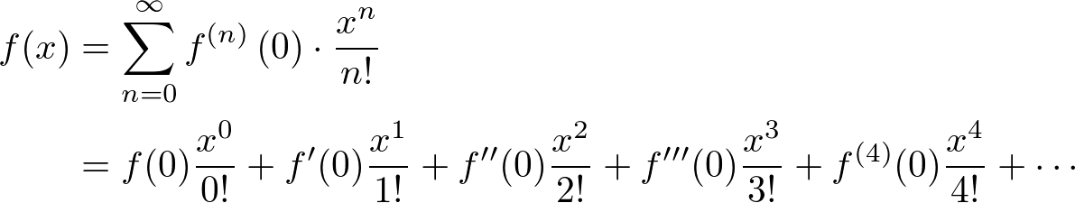
Taylor expansion
Recall first of all the following fundamental "Calculus 1" result: Let $f(x)$ be a smooth function, namely $f(x)$ has derivatives $f^{(n)}(x)$ of every orderand each function $f^{(n)}(x)$ is continuous in $x$. Then, given any point $x_0$, $$ f(x_0+h) = f(x_0) + f'(x_0)h + \frac{f''(x_0)}{2!}h^2+\dots+\frac{f^{(n)}(x_0)}{n!}h^n+\frac{f^{(n+1)}(s)}{(n+1)!}h^{n+1} $$ for every $x$ close enough to $x_0$ and some $s$ between $x_0$ and $x$.
First algorithm for $f'(x)$
Cut the r.h.s. of the formula above after the first two terms. Then we get that $$ f(x_0+h) = f(x_0) + f'(x_0)h + \frac{1}{2}f''(s)h^2 $$ and so thatTruncation error
This formula tells us two important things:- We can approximate the "calculus" limit $f'(x_0)$ with the much simpler "algebraic" rate of change $\frac{f(x_0+h)-f(x_0)}{h}$.
- By doing this, we make an error that, if $f''$ is bounded close to $x_0$, goes to zero at least as fast as the first power of $h=x-x_0$.
in order to find the derivative, we evaluate the fraction above. Point (2) is the truncation error:
the error due to our approximation is equal to a constant times $h$. The smaller $h$, the better the approximation.
Let us test this formula with MATLAB!
The following is a very instructive numerical experiment. We consider the functionLet us test this formula with MATLAB!
(output in the next slide)Better using loglog to plot...
(output in the next slide)What is going on??
We forgot to keep into consideration the round-off error!Let us be more quantitative
In the best case scenario, both $f(x_0+h)$ and $f(x_0)$ have an error of 1 on their last significant digit and so their difference has an error double of that (we must always assume the worst case scenario!). Since the values of the sine function close to $\pi/2$ are about 1,the error
Let us be more quantitative
In our case,What do we learn from here?
The example above shows us clearly one important fact: although it is counter-intuitive, because of the round-off decreasing $h$ beyond some critical value increases the error rather than diminishing it!! In the concrete case discussed above, the smallest error we can achieve is about $10^{-8}$, obtained at $h\simeq10^{-8}$.What if we want to improve our precision?
Unless we can switch to a higher-precision floating system, our best chance to get a smaller error is to use a better algorithm. A simple improvement comes from the following observation: $f(x_0+h) = f(x_0) + f'(x_0)h + \frac{1}{2}f''(x_0)h^2 + \frac{1}{6}f'''(s)h^3$ $f(x_0-h) = f(x_0) - f'(x_0)h + \frac{1}{2}f''(x_0)h^2 - \frac{1}{6}f'''(t)h^3$ soA better algorithm
HenceLet us give it a try...
(output in the next slide)It works!
Another example:
evaluating the value of a function via Taylor expansion.
Evaluating functions via Taylor polynomials
The problem we discuss here is:how to evaluate non-polynomial functions?
For instance, how to evaluate $\cos(0.15)$? This is a problem of continuous mathematics
because $\cos(x)$ is defined over a continuous set
(the real line, or the complex plane if you are brave enough). Polynomial and rational functions can be easily evaluated
using just the four operations,
but what can we do about trascendental functions such as $\cos(x)$?
Taylor expansion
The answer to the question abovecomes from the following theorem: Let $f(x)$ be a $C^\infty$ function,
namely $f(x)$ has derivatives $f^{(n)}(x)$ of every order
and each function $f^{(n)}(x)$ is continuous.
Then, given any point $x_0$, for any other number $x$ and any integer $n$ there is a number $\xi$ between $x_0$ and $x$ such that $$ f(x) = f(x_0) + f'(x_0)(x-x_0) + \frac{f''(x_0)}{2!}(x-x_0)^2+\dots+\frac{f^{(n)}(x_0)}{n!}(x-x_0)^n+\frac{f^{(n+1)}(\xi)}{(n+1)!}(x-x_0)^{n+1} $$
Taylor expansion
The term $$ T_n(x)=f(x_0) + f'(x_0)(x-x_0) + \frac{f''(x_0)}{2!}(x-x_0)^2+\dots+\frac{f^{(n)}(x_0)}{n!}(x-x_0)^n $$ is called the $n$-th Taylor polynomial of $f(x)$ at $x_0$. The term $$ R_n(x) = \frac{f^{(n+1)}(\xi)}{(n+1)!}(x-x_0)^{n+1} $$ is the remainder term. This is not a polynomial termbecause $\xi$ depends, in general, on $x$ in a trascendental way.
An algorithm based on Taylor series
We can use Taylor polynomials to evaluate functionsand then use the remainder term
to evaluate the error due to the approximation. A possible algorithm to evaluate $f(x)$ from a known value $f(x_0)$
with an error not larger than $\varepsilon$ would be the following:
- Determine somehow a $n_0$ such that $|R_{n_0}(x)| < \varepsilon$.
- Evaluate the polynomial $T_{n_0}(x)$.
Example
Let us evaluate $\cos(0.15)$ with an error not larger than $\epsilon=0.00001$.We know the values of the $cosine$ function and all its derivatives at the origin, so we will use $x_0=0$. Clearly, $x=0.15$. Recall that $$\cos'x=-\sin x, \cos''x=-\cos x,$$ $$\cos'''x=\sin x, \cos''''x=\cos x.$$ Hence, the Taylor series of $\cos x$ about $x_0=0$ is $$ 1-\frac{1}{2!}x^2+\frac{1}{4!}x^4-\frac{1}{6!}x^6+\dots+(-1)^n\frac{1}{(2n)!}x^{2n} $$
That $T_4(0.15)$ provides an approximation of $\cos(0.15)$
with an error not larger than $0.00001$. Let's verify this: $$ T_4(0.15) = 1-\frac{x^2}{2}+\frac{x^4}{24}\bigg|_{x=0.15}=0.988771093... $$ An independent estimate of $\cos(0.15)$ with 10 exact digits gives $$ \cos(0.15) = 0.9887710779. $$ Hence actually $$ |\cos(0.15)-T_4(0.15)| = 0.00000001... $$ which is well below $0.00001$.
Remark
So why in the end we got an estimatemuch more precise than we wanted to? Because replacing $|\cos^{(n+1)}(\xi)|$ by 1 was very rough.
For instance, when $n$ is even this derivative is the sine function and we know that $|\sin\xi| < |\xi| < |x|$, namely in this case we could have done the more accurate approximation $$ |R_n(x)|\leq \frac{1}{(n+1)!}x^{n+2} $$ Since $\frac{1}{4!}0.15^{5}<0.000001$, this would have showed us that $n_0=3$ would be enough to get the precision required!
Final comments
There is no general recipe to find the best (or the simplest) upper bound to $|f^{(n+1)}(\xi)|$. The only way to find one is to "give a look" to the derivatives of $f(x)$ and understanding their behavior. This happens very often in numerical analysis: there is no general rule to solve in the optimal way all problems of a certain kind.There are general guidelines but ultimately
each concrete problem needs some litte adjustments.
Root finding methods

A root of a function $f(x)$ is a number $x_0$ such that $$ f(x_0)=0. $$ Besides very few special cases,
the roots of a function can be found only numerically.
Method 1: Bisection
The Bisection Method method is basedon the following fundamental property of continuous functions:
If $f(x)$ is continuous on the interval $[a,b]$ then, between $a$ and $b$, $f(x)$ assumes all possible values
between $f(a)$ and $f(b)$.
In particular, if $f(a)$ and $f(b)$ have opposite signs,
then there is at least a root of $f(x)$ between $a$ and $b$.
The Algorithm
If $f(x)$ is a $C^0$ function and $f(a)$ and $f(b)$ have opposite signs,namely if $f(a)f(b)<0$,
there must be at least a root $x_0$ of $f(x)$ between $a$ and $b$. We have no info on where the root actually is located within the interval $(a,b)$, so which number do we choose as our solution? If we chose $a$ or $b$, in the worst case our error would be $|b-a|$. If we rather choose $m=(a+b)/2$,
then the error cannot be larger than $|b-a|/2$. This is the optimal choice.
The Algorithm
In the same spirit, we can get arbitrarily close to a rootby applying over and over the following elementary step: Define $m=(a+b)/2$.
If $f(a)$ and $f(m)$ have opposite signs,
replace the interval $[a,b]$ with $[a,m]$;
otherwise, replace it with $[m,b]$. This way, at every step we are left with an interval
that does contain for sure a root of $f(x)$
and whose length is half of the previous interval. Hence, after $k$ steps, the error on the position of the root, namely the length of the interval one gets after $k$ iterations, is $|b-a|/2^k$.
Example
Solve numerically the equation $$\cos x=x.$$ This problem is equivalent to finding the root(s) of the function $f(x)=\cos x-x$. In this case it is easy to see that there is a single root.Indeed, since $|\cos x|\leq 1$, there cannot be any root for $x>1$ or $x<-1$. Since $\cos x>0$ for $-\pi/2 < x < 0$,
there cannot be any root in that interval either.
Finally, in the interval $(0,1)$, $\cos x$ is monotonically decreasing
while $x$ is monotonically increasing,
so their graphs can meet there only once.
there is a root of $f(x)=\cos x-x$ between 0 and 1. Let's verify that $f(0)f(1) < 0$: $$ f(0) = \cos0-0=1>0,\;\;f(1)=\cos(1)-1<0 $$ because we know that $\cos0=1$ and that $\cos x$ decreases for $0 < x < \pi$. Hence we set $b=1$ and $a=0$.
At this point, we can say that the solution of $\cos x=x$ is
$x_0=(a+b)/2=0.5$
with an error $\Delta x=|b-a|/2=0.5$
now we know that the solution must be between $0.5$ and $1$.
Hence our new interval is now $[0.5,1]$
(equivalently, we can say that we redefined $a=0.5$). At this point, our best estimate of the root is
$x_0=0.75$
with an error $\Delta x=0.25$.
now we know that the solution must be between $0.5$ and $0.75$.
Hence our new interval is now $[0.5,0.75]$
(equivalently, we can say that we redefined $b=0.75$). At this point, our best estimate of the root is
$x_0=0.625$
with an error $\Delta x=0.125$.
we can get an estimate of the root with any desired precision. For instance, in order to get an estimate of the root with an error not larger than $0.001$, it is enough to use a number of iteration $k$ s.t. $$ |1-0|/2^k < 0.001, $$ namely $$ 1000 < 2^k. $$ You can solve this inequality either with your calculator, noticing that $k>\log_2(1000)\simeq9.97$, or by noticing that $2^{10}=1024$
(a very useful relation to remember).
while on the third digit there is an uncertainty of 1 unit. In case you are curious, the root is equal to $$ x_0=0.739085133\pm0.000000001, $$ which is of course compatible with our rough estimate $$ x_0=0.625\pm0.125. $$
An implementation of the Bisection algorithm
In the code below we evaluate numerically the square root of 2.(the output shows in the slide below)
Output of the code above
(press 'Evaluate' in the previous slide to generate the output)Method 2: Newton's method
The bisection method is very low-demanding: as long as a function is continuous, the method does work and the error decreases linearly. We can improve the convergence speedby asking for more regularity: if we are close enough to a root
the derivative of
The algorithm
Given an initial point $x_0$, the equation of the line tangent to the graph of $f(x)$ passing through $(x_0,f(x_0))$ isDoes it work?
The sequence $x_0,x_1,x_2,\dots$ does not converge necessarily(I'll show an example below)
but if it does, then it does converge to a root. Indeed, assume that
Then, provided that $f$ and $f'$ are continuous and that $f'(r)\neq0$,
We are requiring more regularity to $f$, is it worth?
Unlike the bisection method, Newton's method require the existence and continuity of $f'$.So why do we like it anyways? Speed! The error
decreases quadratically!
An implementation of the Newton's algorithm
The code above evaluates the square root of 2 with Newton's method.(the output shows in the slide below)
Output of the code above
(press 'Evaluate' in the previous slide to generate the output)Method 3: Fixed Point
The Fixed Point Method method is basedon the following fundamental property of differentiable functions:
If $f(x)$ is differentiable with a continuous derivative $f'(x)$ and $x_0$ is a fixed point of $f(x)$, namely $f(x_0)=x_0$, such that $|f'(x_0)|<1$, then the iterates $f(x), f(f(x)), f(f(f(x))),\dots,$ converge to $x_0$ for every $x$ close enough to $x_0$.
Notation: we say that a differentiable functionwith continuous first derivative is a $C^1$ function.
The Algorithm
We are not interested here into fixed points but we want rather to use the fixed point property above to find roots of functions $f(x)$. We accomplish this thanks to the following elementary observation: $x_0$ is a root of $f(x)$if and only if
$x_0$ is a fixed point of the function $g(x)=f(x)+x$.
to estimate the roots of a $C^1$ function $f(x)$.
- transform somehow the equation $f(x)=0$
into a fixed point problem $g(x)=x$; - select somehow an initial point $\hat x$
close to the root $x_0$ you want to evaluate; - evaluate $g(\hat x)$.
and $x$ is "close enough" to $x_0$,
then $g(\hat x)$ will be closer to $x_0$ than $\hat x$
and, by repeating the last step, one can get arbitrarily close to $x_0$.
Example
Let us use the fixed point method to solve the equation $\cos x=x$. Recall that the solution is $ x_0=0.739085133... $ We start by using $g(x)=\cos x$.Let us use as starting point the estimate
we found with the bisection method: $\hat x = 0.625$. Then we find $$ x_1 = 0.810963..., x_2=0.688801..., x_3=0.772009..., x_4=0.716511... $$
The convergence speed is not very good, in 4 steps we get only the first digits right. The reason is that $$ |g'(x_0)|\simeq0.67, $$ namely with this choice
the fixed point method is actually slower than the bisection one.
For instance, $\cos x-x=0$ is equivalent to $\cos x-x+x^2=x^2$ and so to $\pm\sqrt{\cos x-x+x^2}=x$. Hence, we can use $g(x)=\sqrt{\cos x-x+x^2}$.The first four terms of the sequence are
$$ x_1= 0.759333..., x_2=0.736579..., x_3=0.739419..., x_4=0.739041... $$ In this case, we get a new correct digit at every iteration.
The reason is that now $$|g'(x_0)|\simeq0.13$$
Bisection vs Fixed Point
The fixed point method requires more regularitythan the bisection method ($f(x)$ must be $C^1$ rather than $C^0$)
and it is not guaranteed to converge, while the bisection method is. So... why on earth would someone want
to use the latter rather than the former??? The answer is: speed.
Convergence speed of the bisection method
Consider the sequence of estimates $x_1,x_2,\dots$, coming from an application of the bisection method. The error of $x_k$ is given by $\Delta x_k=|b-a|/2^k$, where $b$ and $a$ are the endpoints of the initial segment. So $$ \Delta x_{k+1}/\Delta x_k=1/2, $$ namely the error decreases by a fixed amount. We say that this sequence converges to the solution with order 1.Convergence speed of the fixed point method
Consider now the case of the fixed point method. Since $|f'(x_0)| < 1$, the rate of change of $f(x)$ for every $x$ close enough to $x_0$ satisfies $$ \bigg|\frac{f(x)-x_0}{x-x_0}\bigg| < M $$ for some number $M < 1$. This means that $$ \Delta x_{k+1} = |x_{k+1}-x_0| < M |x_k-x_0| = M \Delta x_k, $$ since in the fixed point method $x_{k+1}=f(x_k)$. Hence, here, $$ \Delta x_{k+1}/\Delta x_k=M. $$the method switches from order 1 to order 2.
This (see the discussion about the Newton method) means that its speed increases significantly.
A crash course in
Linear Algebra

Linear Functions
Consider a function in 1-variable $f(x)$.What do we mean by saying that $f(x)$ is a linear function?
Definition:
$f(x)$ is linear if- $f(x+y)=f(x)+f(y)$ for all real numbers $x,y$;
- $f(s\cdot x)=s\cdot f(x)$ for all real numbers $s,x$.
Linear Functions in 1 variable
So... what does a linear function look like?From the definition, $$ f(x) = f(x\cdot1)=xf(1)=a x, $$ where $a=f(1)$. Yes, linear functions are simply polynomials of degree 1
without the constant term.
Linear Functions in 2 variables
How to generalize linearity to functions in several variables?Consider first the case of two real variables $x,y$. Recall that, as $x$ and $y$ assume all their possible values, the ordered pair $(x,y)$ represents, exactly once, every single point on the plane. Points $(x,y)$ on the plane can be considered as vectors
and so can be summed and scaled, i.e. multiplied by a scalar: $$ (x,y)+(x',y') = (x+x',y+y'),\;\;s\cdot(x,y) = (s\cdot x,s\cdot y) $$ for all points $(x,y),(x'y')$ and all scalars $s$.
Linear Functions in 2 variables
Now that we know what does it mean to sum and to scale,we can say what is a linear function in 2 variables:
Definition:
$f(v)$, where $v=(x,y)$, is linear if- $f(v+v')=f(v)+f(v')$ for all pairs $v=(x,y)$, $v'=(x',y')$;
- $f(s\cdot v)=s\cdot f(v)$ for all scalar $s$ and for every point $v=(x,y)$.
Yes, it looks exactly like the definition for functions of 1-variable, except that here the argument of the function
is a point on the plane rather than a point on a line.
Linear Functions in 2 variables
Ok, but so what does a linear function in two vars look like? Similarly to the 1-var case (but here we do need property 1!)Matrix Notation in 2 variables
People found out that it is very convenientwriting linear functions in matricial notation. A point $v=(x,y)$ is written as a column matrix:
Linear Functions in $n$ variables
Now we can write the general case of $n$ variables.In this case, points $v$ are $n$-tuples of real numbers $(x_1,\dots,x_n)$.
Definition:
$f(v)$, where $v=(x_1,\dots,x_n)$, is linear if- $f(v+v')=f(v)+f(v')$ for all points $v=(x_1,\dots,x_n)$, $v'=(x'_1,\dots,x'_n)$;
- $f(s\cdot v)=s\cdot f(v)$ for all scalar $s$ and for every point $v=(x_1,\dots,x_n)$.
Linear Functions in $n$ variables
Just as in case of two variables, $$ f(x_1,\dots,x_n) = a_1 x_1+\dots+a_n x_n, $$ where $$ a_1 = f(1,0,\dots,0), $$ $$ a_2 = f(0,1,0,\dots,0), $$ $$ \vdots $$ $$ a_n = f(0,\dots,0,1). $$Matrix Notation in $n$ variables
A point $v=(x_1,\dots,x_n)$ is written as a column matrix:Linear Maps
The space of vectors with 2 real components is denoted by $\Bbb R^2$.Take two linear functions in two variables $f(x,y)$ and $g(x,y)$.
With them, we can define a map $F$ of the plane into itself: $$ F(x,y)=(f(x,y),g(x,y)). $$ Since its components are linear, this map is called linear too.
whose rows are exactly the matricial representations of $f$ and $g$: $$ F(v) = \pmatrix{a & b\cr c&d\cr}\cdot\pmatrix{x\cr y} = \pmatrix{a x+b y\cr cx+dy\cr}, $$ where $v$ is the point $(x,y)$.
General linear maps
The space of vectors with $n$ real components is denoted by $\Bbb R^n$.Linear functions therefore are maps $f:\Bbb R^n\to\Bbb R$. In general, we can have $m$ linear functions $f_i$ in $n$ variables $x_j$.
Put together, the functions $f_j$ define a linear map $F$ from $\Bbb R^n$ to $\Bbb R^m$: $$ F(x_1,\dots,x_n)=(f_1(x_1,\dots,x_n),\dots,f_m(x_1,\dots,x_n)). $$
General linear maps as matrices
Let us use the following notation: $$ f_1(x_1,\dots,x_n)=a_{11}x_1+a_{12}x_2+\dots+a_{1n}x_n, $$ $$ f_2(x_1,\dots,x_n)=a_{21}x_1+a_{22}x_2+\dots+a_{2n}x_n, $$ $$ \vdots $$ $$ f_m(x_1,\dots,x_n)=a_{m1}x_1+a_{m2}x_2+\dots+a_{mn}x_n. $$General linear maps as matrices
Then, in matrix notation,This is a rectangular matrix with $n$ columns and $m$ rows. In this course, we are interested only in the case $m=n$.
Matrices with equal number of rows and columns are called
square matrices.
Matrices
Why do we care about matrices?Consider the $3\times3$ linear system $$ \left\{ \begin{aligned} 2x+3y-z&=1\cr \phantom{2x+}y+3z&=0\cr 7x+y-2z&=5\cr \end{aligned} \right. $$ With matrices, we can rewrite the system as $$ \pmatrix{2&3&-1\cr 0&1&\phantom{-}3\cr 7&1&-2\cr } \cdot \pmatrix{x\cr y\cr z\cr} = \pmatrix{1\cr 0\cr 5\cr}. $$
Matrices help solving linear systems
Rewriting in sysmbols the matricial equation as $$ A\cdot v=w $$ suggests that, if there were possible to "divide by $A$",we could solve the equation as for real numbers: $$ v = w/A . $$ In order to have "inverse matrices",
there must be a product of matrices.
This is what we do below.
Product of $2\times2$ Matrices
Take two linear maps from the plan to itself:Product of $2\times2$ Matrices
We use exactly this formula to define the product of $2\times2$ matrices: $$ \begin{pmatrix}a&b\cr c&d\cr\end{pmatrix}\cdot\begin{pmatrix}p&q\cr r&s\cr\end{pmatrix} = \begin{pmatrix}ap+br&aq+bs\cr cp+dr&cq+ds\cr\end{pmatrix} $$ Observe that the rule is a straightforward generalizationof the product of a matrix by a column vector. In this case, though, since the right matrix is made of two columns,
the outcome is two columns rather than one, namely a $2\times2$ matrix.
Index Notation
Since we are going to write formulas for a general "$n\times n$" matrix,we need to learn how to write this product a bit more abtractly. Let us start with the $2\times2$ case:
Matrix Product
The formula above is exactly what we needto write concisely the product of $n\times n$ matrices. Given two $n\times n$ matrices $A=(a_{ij})$ and $B=(b_{ij})$, $1\leq i,j\leq n$, the entry $ij$ of the product are given by the formula $$ (A\cdot B)_{ij} = a_{i1}b_{1j}+\dots+a_{in}b_{nj}=\sum_{k=1}^n a_{ik}b_{kj}. $$
Invertible Matrices
So... how to find the inverse $A^{-1}$ of a matrix $A$? Well, the formula is a bit complicatedbut the main reason why I won't go over it is that... we won't need it. A great explanation of why we won't need it
is the following observation by Forsythe and Moler: Almost anything you can do with $A^{-1}$, can be done without it. The main reason why we don't want to evaluate $A^{-1}$
is that it involves the evaluation of the determinant of $A$.
Determinant of a $2\times2$ Matrix
Notice the following fact: $$ \begin{pmatrix}a&b\cr c&d\cr\end{pmatrix}\cdot\begin{pmatrix}1\cr 0\cr\end{pmatrix} = \begin{pmatrix}a\cr c\cr\end{pmatrix}, \; \begin{pmatrix}a&b\cr c&d\cr\end{pmatrix}\cdot\begin{pmatrix}0\cr 1\cr\end{pmatrix} = \begin{pmatrix}b\cr d\cr\end{pmatrix}. $$ This shows that the columns of the $2\times2$ matrixof a linear map $F$ have a meaning:
they are the vectors images of the basic vectors $\begin{pmatrix}1\cr 0\cr\end{pmatrix}$ and $\begin{pmatrix}0\cr 1\cr\end{pmatrix}$.
The vectors $\begin{pmatrix}a\cr c\cr\end{pmatrix}$ and $\begin{pmatrix}b\cr d\cr\end{pmatrix}$ are two of the four sides of a parallelogram $P$. In other words, $P=F(\text{unit cube})$.
The (signed) area of $P$ is called the determinant of $A$.
As you may know already, in concrete $\det A=ad-bc$.
Determinant of a $n\times n$ Matrix
The definition of the determinant of a $n\times n$ matrix $A$of a linear map $F$ of $\Bbb R^n$ into itself is completely analogous. The $n$ columns of $A$ are the images
of the unit positive vectors on the $n$ coordinate axes. The determinant of $A$ is the "$n$-dimensional" volume of the $n$-dimensional parallelogram $P$, $n$ sides of which are the $n$ columns of $A$. In other words, $P=F(\text{unit $n$-dimensional cube})$ Note that, since $F$ is linear, this also means that, given any region $R$, $$ \text{Area}(F(R)) = \det A\cdot\text{Area}(R), $$ namely $\det A$ is the area scaling factor of $F$.
Determinant of a $n\times n$ Matrix
The problem with the determinantis that it entails a number of calculations larger than $n!$. Notice that $100!\simeq10^{158}$, namely calculating the determinant of a $100\times100$ matrix is going to take a really long time. The current fastest supercomputer is able to perform about $0.5\times 10^{18}$ floating-point operations per second. For instance, evaluating the determinant of a $30\times30$ matrix
directly from the definition
would take in general more than 6 millions years.
Unit Matrix
Is it evaluating determinants so hard for every matrix?Of course not! A simple example is the determinant of the identity map: $$I(v)=v.$$ The corresponding matrix, for instance in case $n=3$, is 1$_3 = \begin{pmatrix}1&0&0\cr 0&1&0\cr 0&0&1\cr\end{pmatrix}$ Clearly, the image of the $n$-dimensional cube through $I$ is itself,
and therefore $\det($1$_n)=1$.
Diagonal Matrices
More generally, a linear map is diagonalif its action on the coordinate vectors is a scaling. For instance, in case of $3\times3$ matrices, $F$ is linear if the corresponding matrix $A$ satisfies the following:
is a cuboid of sides $\alpha$, $\beta$ and $\gamma$. Hence, $\det A = \alpha\beta\gamma$.
Diagonal Matrices
This is true for every $n$: given a diagonal $n\times n$ matrix $A$with scaling factors $\alpha_1,\dots,\alpha_n$, $$ \det A = \alpha_1\cdots\alpha_n. $$
Upper and Lower triangular Matrices
A matrix is upper triangular if all terms below the diagonal are 0.For instance, below is a $3\times3$ upper triangular matrix: $$ A = \begin{pmatrix} 3&2&-1\cr 0&-1&7\cr 0&0&13\cr \end{pmatrix}. $$ Simple geometrical considerations, especially simple in the 2- and 3-dimensional case, show that the the determinant of an upper triangular matrix is equal to the determinant of the diagonal matrix with the same diagonal entries. For instance, $\det A=3\cdot(-1)\cdot13 = -39$.
The same can be said for lower triangular matrices.
Norms on Vector Spaces
A norm on a linear space $\Bbb R^n$ is a map $\|\cdot\|:\Bbb R^n\to[0,\infty)$ s.t.- $\|x\|>0$ if $x\neq0$;
- $\|\lambda x\|=|\lambda|\cdot\|x\|$ for all scalars $\lambda\in\Bbb R$;
- $\|x+y\|\leq\|x\|+\|y\|$.
- $\|x\|_1 = \sum_{i=1}^n |x^i|$; (see Taxicab norm)
- $\|x\|_2 = \sqrt{\sum_{i=1}^n |x^i|^2}$; (the ususal Euclidean norm)
- $\|x\|_\infty = \max_{i}|x^i|$. (Chebyshev distance)
What is the meaning of the norms other than Euclidean?
The norm of a vector with endpoints $A$ and $B$is also the distance between point $A$ and point $B$
and the concept of distance depends on the environment. For instance, if points $A$ and $B$ are two points in an ice ring, definitely the most suitable concept of distance is the Euclidean one:
one just moves from $A$ to $B$ on the straight line joining them. But if the two points mark two buildings in Manhattan, then to go from $A$ to $B$ you can not move diagonally (you'd cross the buildings) but only either horizontally or vertically,
so you should use the Taxicab norm. But if $A$ marks a King piece on a chessboard, which can also move diagonally, then the number of moves it takes to the King to get to $B$ is given by the Chebyshev distance between $A$ and $B$!
Does "being small" differ from norm to norm?
Quantitatively: YES. For instance, the set of all vectors of norm 1 is different in all three norms above. Consider just the plane:- The taxicab unit circle $|x|+|y|=1$ is a square of side $\sqrt{2}$ with sides parallel to the bisetrices of the quadrants.
- The Euclidean unit circle $x^2+y^2=1$ is just the usual circle.
- The Chebyshev unit circle $\max\{|x|,|y|\}=1$ is a square of side 2 with sides parallel to the coordinate axes.
Norms of Matrices
The set of $n\times n$ matrices $M_n(\Bbb R)$ is a vector space itself and so it makes sense to speak about the norm of its elements. A very improtant norm is the one it inherits from the space it acts upon: $$ \|A\| = \sup_{x\neq0}\frac{\|Ax\|}{\|x\|} $$ Examples:- $\|A\|_1 = \max_{j}\sum_{i=1}^n |A^i_j|$;
- $\|x\|_2$ is the maximum eigenvalue of $\sqrt{A^*A}$;
- $\|A\|_\infty = \max_{i}\sum_{j=1}^n |A^i_j|$.
An important property
For all norms above, $$ \|A\cdot B\|\leq \|A\|\cdot\|B\| $$ (namely the product is a continuous operator!).Solving numerically linear systems

1. The LU method
Ok, so how do we solve the linear system $Ax=b$ without $A^{-1}$?? There are several ways. Here we cover the oldestand most well known method, called the LU Method. The trick here is to write $A$ as the product
of a lower triangular matrix $L$ times an upper triangular matrix $U$. How does this help? The point is that, if $A=L\cdot U$, $$A^{-1}=(L\cdot U)^{-1} = U^{-1}\cdot L^{-1}.$$ Since the determinant of $U$ and $L$ are easy to compute, it is reasonable that this method is much faster than the naif one.
An implementation of the LU algorithm
(the output shows in the slide below)Output of the code above
(press 'Evaluate' in the previous slide to generate the output)Another implementation of the LU algorithm
This implementation is a bit fancier: code checks whether the matrix $A$ is a square matrix (line 4)and whether the pivot element is diving for is non-zero (line 7).
Moreover, we avoid a for loop by using some fancy MATLAB capability.
(the output shows in the slide below)
Computational Complexity of the LU algorithm
We want to evaluate the order of magnitude of how many calculations are needed to perform a LU decomposition of a $n\times n$ matrix $A$. This is called the computational complexity of the algorithm. In general, the answer is a polynomial in $n$ of some degree. We do not need the exact number, only the degree of the polynomial, namely we want to know whether this number scales like $n^2$ or $n^3$ and so on. According to the algorithm, at the first step we do one division(to find $L(i,j)$),
$n$ multiplications
(when we multiply the first row by $L(i,j)$)
and $n(n-1)$ subtractions
(when we subtract the 'normalized' first row
from the remaining $n-1$ ones).
Computational Complexity
(the output shows in the slide below)The code below counts the number of operations needed for
the LU decomposition of a matrix for $n$ between 1 and 20
and plots the result in a log-log plot.
Output of the code above
(press 'Evaluate' in the previous slide to generate the output)Problems of the LU algorithm
The elementary implementation above suffers two main problems:- It fails if the element
A(j,j) is zero when we evaluateL(i,j) . - There might be a loss of significant digits in the difference
A(i,k)-L(i,j)*A(j,k) ifL(i,j) is very big.
Example: applying the algorithm to
as if the original matrix were
A concrete example
Let us make concrete calculations in an example in the floating point system $F$ with base 10 and three significant digits. Consider the system $$ Ax=b $$ $$ \begin{pmatrix} 0.00025&1\\ 1&1\\ \end{pmatrix} \begin{pmatrix} x\\ y\\ \end{pmatrix} = \begin{pmatrix} 1\\ 2\\ \end{pmatrix} $$ Its exact solution is $x=\frac{4000}{3999},y=\frac{3998}{3999}$, both equal to $1.00$ in $F$.A concrete example
Using the LU decomposition, though, we getA concrete example
In other words, the system is equivalent to $$ \left\{ \begin{array}{c} 0.00025x+y=1\\ -4000y=-4000\\ \end{array} \right. $$ so that $y=1.00$ and therefore $x=0.00$. Notice that we got a relative error of 100% in $x$!!!Pivoting
This kind of problems can be fixed by rearranging at every step the rows of $A$ so that, when we evaluateby applying it to the system of the previous example:
so we re-write it as
The error we experienced before pivoting disappeared completely!
Error Analysis
The $n\times n$ symmetric matrices defined by $A^i_j = \frac{1}{i+j-1}$ do not behave well under $LU$ decomposition (check by examples!). In order to be able to say in advance when a matrix will be not easy to treat numerically, it was introducted by Alan Turingthe concept of conditioning of a (non-singular) matrix: $$ k(A) = \|A\|\cdot\|A^{-1}\|, $$ where $\|A\|$ is some norm of $A$ (it does not really matter which one!).
Conditioning
Cearly the conditioning depends on the norm used but its asymptotic behavior does not since, in finite dimension, all norms are equivalent! Geometrically, the conditioning of $A$ is the ratio betweenthe maximum relative stretching on a vector
and the maximum relative shrinking. Since $k(\Bbb I_n)=1$ in any of such norms, then $$ 1=\|{\Bbb I}_n\| = \|AA^{-1}\|\leq\|A\|\cdot\|A^{-1}\|=k(A). $$ Moreover, $k(\lambda A)=k(A)$ and, for a diagonal matrix, $k(A)=\max|d_i|/\min|d_i|$.
Error propagation
Let $\hat x=x+\Delta x$ be the solution of $Ax=b+\Delta b$.Since $A$ is linear, $$ A\hat x = A(x+\Delta x)=Ax+A\Delta x=b+\Delta b, $$ so $A\Delta x = \Delta b$. Hence $\|b\|\leq\|A\|\cdot\|x\|$ and $\|\Delta x\|\leq\|A^{-1}\|\cdot\|\Delta b\|$, so that
Ill Conditioned matrices
When $k(A)$ is "close to 1" we say that $A$ is well conditioned, otherwise we say that it is ill conditioned. Hilbert matrices are a good example of very ill conditioned matrices:
      >> hilb(3)
				   ans =
				   1.0000    0.5000    0.3333
				   0.5000    0.3333    0.2500
				   0.3333    0.2500    0.2000
				   >> cond(hilb(3))
				 ans =
				 524.0568
				 >> hilb(4)
		ans =
		1.0000    0.5000    0.3333    0.2500
		0.5000    0.3333    0.2500    0.2000
		0.3333    0.2500    0.2000    0.1667
		0.2500    0.2000    0.1667    0.1429
		>> cond(hilb(4))
	      ans =
	      1.5514e+04
Residual
The residual of a numerical solution of a linear equation is $$ r=b-A\hat x $$ In principle it is a good estimator of the quality of the solutionbut it actually depends on the conditioning of $A$! $$ \frac{\|\Delta x\|}{\|x\|}\leq k(A)\frac{\|r\|}{\|b\|} $$ so
if $k(A)$ is very large
we can have very imprecise solutions
even in presence of very small residuals.
Example
In 4-digits decimal arithmetic,let us use the LU method for the linear system
with only one significant digit left,
so that only the order of magnitude of $y$ is correct. When $y$ is used to determine $x$, we get a small residual only because $A$ shrinks a lot exactly in the direction of $r$,
but clearly we can trust no more than a single digit of this $x$.
2. Fixed-Point Methods
Just like in case of equations in one variable,$n\times n$ linear systems can be solved by iteration methods. The main idea of these methods can be illustrated
in the elementary case of linear equations in one variable. Re-write $ax=b$ as $x=(1-a)x+b$a.
Hence, a solution of $ax=b$ is a fixed point of $$g(x)=(1-a)x+b.$$ When is this point attractive?
We know it: $g'(x)=1-a$, so it is attractive when $|1-a| < 1$.
no matter what is the value of $x_0$. We can repeat this for any $n\times n$ non-degenerate linear system $$ Ax=b. $$ We re-write the system as $x = ($1$_n-A)x+b$, where 1$_n$ is the identity matrix,
so that the solution is a fixed point of the linear map $g(x) = ($1$_n-A)x+b$.
of the sequence above is that $\|$1$_n-A\|<1$. EXAMPLE: let us apply this naif method to the system
Jacobi and Gauss-Seidel Methods
Adding 1$_n$ to both sides is not optimalbecause the condition $\|$1$_n-A\|<1$ is quite strict. In general, one adds $Qx$ to both sides and then "divides by $Q$",
so that the iterating function is $g(x) = $(1$_n-Q^{-1}A)x+Q^{-1}b$ The following two alternate choices are often used:
- $Q=diag(A)$ (Jacobi method);
- $Q=tril(A)$ (Gauss-Seidel method)
Example
Consider the system$$ \begin{pmatrix} 3&1\\ 2&4\\ \end{pmatrix} \begin{pmatrix} x\\ y\\ \end{pmatrix} = \begin{pmatrix} 4\\ 6\\ \end{pmatrix}, $$
By solving w/resp to $x$ the first and to $y$ the second we get that $$ \begin{cases} 3x &= -y+4\\ 4y &= -2x+6\\ \end{cases} $$ The solution of the system is $x=1, y=1$.chosen any point $(x_0,y_0)$, we set $$ \begin{cases} 3x_{k+1} &= -y_k+4\\ 4y_{k+1} &= -2x_k +6\\ \end{cases} \; \hbox{(Jacobi method)} $$ or $$ \begin{cases} 3x_{k+1} &= -y_k+4\\ 4y_{k+1} &= -2x_{k+1}+6\\ \end{cases} \; \hbox{(Gauss-Seidel method)} $$
Example
Example
When to use iterative methods
In case of large systems, iterative methods can be more efficientthan direct methods such as the LU decomposition.
Eigenvalues and Eigenvectors
of a Linear Operator
Eigenvalues and Eigenvectors
Main question: How many essentially different behaviorscan a linear operator $f$ have? Consider for example the simplest case, namely dimension 2. Remember that an operator $f$ is completely determined
by what it does on the vector basis $\{e_1,e_2\}$: $$ f(\lambda e_1+\mu e_2) = f(\lambda e_1)+f(\mu e_2) = \lambda f(e_1)+\mu f(e_2) $$ There are just 3 possibilities. The map $f$ can either leave invariant:
- two directions; or
- one direction; or
- none at all.
Two invariant directions
Choose $e_1$ and $e_2$ as vectors pointing in those two directions.Then $$ f(e_1)=\lambda_1e_1\hbox{ and }f(e_2)=\lambda_2e_2 $$ In other words, in this basis $f$ is represented by the matrix $$ \begin{pmatrix}\lambda_1&0\cr0&\lambda_2\cr\end{pmatrix} $$ The numbers $\lambda_1$ and $\lambda_2$ are called eigenvalues of $f$
and $e_1$ and $e_2$ the corresponding eigenvectors. IMPORTANT: eigenvalues are uniquely determined, eigenvectors are just determined up to a non-zero multiplicative constant, namely what is uniquely detemrined is the eigendirection.
Only one invariant direction
Choose $e_1$ and $e_2$ as vectors pointing in those two directions.Then $$ f(e_1)=\lambda e_1\hbox{ and }f(e_2)=\alpha e_1+\beta e_2. $$ If $\beta\neq\lambda$, then the direction $e'_2=e_1+\frac{\alpha}{\beta-\lambda}e_2$ would also be invariant (check it!), against our assumption, so actually $$ f(e_1)=\lambda e_1\hbox{ and }f(e_2)=\alpha e_1+\lambda e_2. $$ Moreover, with a similar change of base we can always have $\alpha=1$, namely in such basis $f$ is represented by the matrix $$ \begin{pmatrix}\lambda&0\cr1&\lambda\cr\end{pmatrix} $$
No invariant direction
You know already a kind of linear transformationsthat leave no direction invariant: rotations! In fact, in some appropriate basis,
every linear operator $f$ with no invariant direction writes as $$ \lambda\begin{pmatrix}\cos\theta&-\sin\theta\cr\sin\theta&\phantom{-}\cos\theta\cr\end{pmatrix} $$ namely it is a roation by an angle $\theta$ composed with a stretch of $\lambda$. In complex numbers notation, the action on the plane of this matrix
is a multiplication by the complex number $\lambda e^{i\theta}$.
The $n$-dimensional case
These three cases represent actuallyall that can happen to a linear operator in any dimension namely: given any operator $f$ on $\Bbb R^n$, we can always split $\Bbb R^n$
in smaller invariant subspaces where $f$ either:
- is diagonal (namely has a number of eigendirections equal to the dimension of the subspace, like case 1);
- has a single eigendirection (like case 2);
- has no eigendirection (and then is it like case 3).
Important facts
- Since multidimensional rotations always break down to compositions of 2-dimensional rotations, an operator on an odd-dimensional vector space has always at least one real eigenvalue.
- Symmetric matrices have always all real eigenvalues.
- More generally, normal operators, namely such that their matrix $A$ satisfies $AA^T=A^TA$, have all real eigenvalues.
The Power method
The most common situation in applications is the determination of the eigenvalues of some symmetric positive-definite matrix,so from now on we assume we have such a matrix. The power method is a very simple iterative method able to evaluate numerically the largest eigenvalue of a matrix $A$
(and so also the smallest, taking $A^{-1}$). Denote by $\{e_1,\dots,e_n\}$ a (unknown!) basis of eigenvectors, so that $Ae_i=\lambda_ie_i$, and take a generic vector $v=v_1e_1+\dots+v_ne_n$ (generic means that no $v_i$ component is zero). Then $$ A^k(v) = v_1\lambda^k_1e_1+\dots+v_n\lambda^k_ne_n $$
The algorithm
If it happens that $\lambda_n$ is larger than all other eigenvalues, then $A^k(v)\simeq\lambda^k_ne_n$ and this approximation gets better and betterwith higher and higher powers of $A$.
We exploit this fact in the following iterative algorithm:
- Choose a random vector $v_0$ and set some threshold $\epsilon$;
until $\|v-vold\|>\epsilon$
$vold = v$
$z = Av$
$v = z/\|z\|$end
At the end of the loop,
$\lambda=\frac{v^TAv}{v^Tv}$ is the eigenvalue of highest modulus
and $v$ an eigenvector with eigenvalue $\lambda$. In essence, this is exactly the method used by google to rank
web pages when a user searches for keywords.
An example
Optimization

What does it mean optimizing a function
Optimizing a function $f:\Bbb R^n\to\Bbb R$ means finding its extrema,namely its local maxima and minima.
Since a max of $f(\boldsymbol{x})$ is a min for $g(\boldsymbol{x})=-f(\boldsymbol{x})$,
we will consider just the case of a local minimum. Recall that the extrema of a function $f(\boldsymbol{x})$ with continuous first derivative are all zeros of the gradient $\nabla f(\boldsymbol{x})$,
which is a vector with $n$ components. Hence solving an optimization problem of a smooth function is equivalent to solving a system of $n$ equations in $n$ variables. IMPORTANT: in a local min, the Hessian matrix is positive-definite.
Example
If $f(x)$ is quadratic, it can be written in matrix notation as $$ f(x) = \frac{1}{2}\boldsymbol{x}^TA\boldsymbol{x} - b^T\boldsymbol{x} +c $$ where $A$ is a $n\times n$ symmetric matrix,$b$ a vector with $n$ components
and c a number. $f(x)$ has a minimum if and only f all eigenvalues of $A$ are positive Exercise: write down explicitly the case $n=2$. Then $\nabla f(x) = A\boldsymbol{x} - b$, so the position of the minimum is the solution of the linear system $A\boldsymbol{x}=b$!
Iterative methods
These are popular methods to findmaxima and minima of functions. Moreover, at the same time,
they also work as methods to solve linear and nonlinear systems! They work as follows: start with some $\boldsymbol{x_{0}}$, that must be decided after some study of the functions (there is no universal recipe!)
and at every step $k$ determine a direction $\boldsymbol{d}_k$
and a number $\alpha_k$ so that the new point $ \boldsymbol{x_{k+1}}=\boldsymbol{x}_k+\alpha_k \boldsymbol{d}_k $ gets closer and closer to the minimum $\boldsymbol{\bar x}$.
Gradient methods
Recall that the gradient $\nabla_\boldsymbol{x}f$ points at each pointat the direction of maximal growth of $f$ at $\boldsymbol{x}$.
Then is a good choice setting $ \boldsymbol{d}_k = - \nabla_\boldsymbol{x_k}f $ More generally, one can set $ \boldsymbol{d}_k = - C_k\nabla_\boldsymbol{x_k}f $ as long as every $C_k$ is a positive-definite matrix,
namely $C_k$ is symmetric
and all of its eigenvalues are positive for every $k$.
How to choose $d_k$?
Steepest descent method $ \boldsymbol{d}_k = - \nabla_\boldsymbol{x_k}f $ Newton method $ \boldsymbol{d}_k = - Hess_{x_k}(f)^{-1}(\nabla_\boldsymbol{x_k}f) $ This last method is the $n$-dimensional analogueof the Newton method we already met in dimension 1.
How to choose $\alpha_k$?
There are many possible choices,below are a few simple ones:
- constant step size: $\alpha_k=s$
- might not converge is $s$ is too large, might be slow if $s$ is too small.
- diminishing size: $\alpha_k\to0$, e.g. $\alpha_k=1/k$
- should not converge to 0 too fast or might be slow.
- line search: $\alpha_k$ minimizes $g_k(\alpha)=f(x_k+\alpha d_k)$
- can use 1-dim root-finding methods to get $\alpha_k$;
Stopping Criteria
There are several possible stopping criteria for these methods. Let $\epsilon>0$ be a given threshold:- $\|\nabla_{x_k} f\|<\epsilon$ (we got close enough to a critical point).
- $\|f(x_{k+1})-f(x_k)\|<\epsilon$ (the value of $f$ stabilized).
- $\|x_{k+1}-x_k\| < \epsilon$ (iterates stabilized).
- $\frac{\|f(x_{k+1})-f(x_k)\|}{\max\{1,\|f(x_k)\|\}}<\epsilon$ (the relative change in $f$ is stabilizing).
- $\frac{\|x_{k+1}-x_k\|}{\max\{1,\|x_k\|\}}<\epsilon$ (the relative change in $x$ is stabilizing).
Steepest Descent
Pseudo-code
Let us see some pseudo-code for the steepest descent algorithmwith linear search in case of quadratic functions:
- select an initial point $x$;
- select a threshold $\epsilon>0$;
- until $\|\nabla_{x}f\|<\epsilon$:
$x\to x-\frac{\nabla_{x}f^T\nabla_{x}f}{\nabla_{x}f^T\,A\,\nabla_{x}f}\nabla_{x}f$. - print $x$.
A concrete implementation
Same code + plots
Convergence
Are these methods going to converge?In some case,
at least ignoring the computational errors,
the answer is positive: THEOREM
- the smallest eigenvalue of the $C_k$ is not approaching 0;
- the setpsize is chosen according to the minimization rule;
namely $\nabla_{x^*}f=0$.
it could be a saddle point of a local max! In case $f$ is quadratic, though, there is only one critical point... THEOREM
Let $f(x)=\frac{1}{2}x^TAx+b^Tx+c$, with $A$ symmetric and with all positive eigenvalues, and let $x^*$ be the position of its minimum.
Then, for the steepest descent method:
- with $\alpha_k$ given by line search, $x_k\to x^*$ for all initial points;
- with fixed step size $\alpha$, the same happes provided that $\alpha<2/\lambda_Q$, where $\lambda_Q$ is the largest eigenvalue of $Q$.
Rate of Convergence
We say that $x_k\to x^*$ with order $p$ if, from some $k_0$ on, $$ \|x_{k+1}-x^*\|\leq c\|x_k-x^*\|^p $$Let $f(x)=\frac{1}{2}x^TAx+b^Tx+c$, with $A$ symmetric and with all positive eigenvalues, and let $x^*$ be the position of its minimum.
Then the sequence $x_k$ generated by the steepeset descent method with exact line search converges to $x^*$ linearly with
$c=\frac{k(A)-1}{k(A)+1}$. Hence, if $k(A)=1$ then the convergence is actually quadratic.
If $k(A)$ is close to 1, the convergence is fast while,
if $k(A)$ is large, the convergence gets slower and slower:

Newton's Method
Newton's method looks for an optimal point $x^*$ of $f(x)$by looking for a zero of the gradient vector field $\nabla_x f$.
Its formulation, like in the 1-dim case, comes from Taylor's expansion: $$ \nabla_{y}f \simeq \nabla_{x} f + Hess_{x}f\cdot(y-x) $$ so, in order to have $\nabla_{y}f=0$, the best bet is choosing $y$ so that $$ y = x - (Hess_{x}f)^{-1}\cdot(\nabla_{x} f) $$ Like in the 1-dim case, Newton's method converges in a single step when $f(x)$ is quadratic -- this is not very surprising:
when $f(x)=x^TAx+b^Tx+C$, its Hessian $Hess_{x}f$ is constant and equal to $A$ and to use Newton's method we need to evaluate $A^{-1}$, which amounts to solving the linear system $Ax=-b$.
Pseudo-code
- select an initial point $x$;
- select a threshold $\epsilon>0$;
- until $\|\nabla_{x}f\|<\epsilon$:
$x\to x-(Hess_{x}f)^{-1}\cdot(\nabla_{x}f$). - print $x$.
A concrete implementation
Convergence
Does this method always converge?Short answer: No.
Nicer answer: Yes, provided that we start "close enough". THEOREM
Then there is some distance $\epsilon>0$
such that the Newton method converges to $x^*$
for every initial point $x_0$ whithin $\epsilon$ from $x^*$.
that are further away: they may or may not converge. REMARK 2. This method just looks at zeros of the gradient,
so there is guarantee that this point is a minimum:
it could be a saddle or even a maximum!
Rate of Convergence
THEOREM:Newton's method converges quadratically.
Conjugate Gradient
A shortcoming of the steepest descent method is that it tends to "zig-zag" a lot, namely we come back often to the same (or almost the same) direction many times. It would be much faster if we could find a set of directions that avoids this. A natural fix to this problem is choosing the sequence of the $\boldsymbol{p}_{k+1}$ as vectors that are "$A$-orthogonal", namely $$ \boldsymbol{p}_{k+1}^T\cdot A\boldsymbol{p}_j=0\,,\;j=0,\dots,k, $$ starting with the usual $\boldsymbol{p_0}=\nabla_{\boldsymbol{x_0}}f$.Conjugate Gradient's Algorithm
Assume that $f(\boldsymbol{x})\simeq\frac{1}{2}\boldsymbol{x}^TA\boldsymbol{x}-b^T\boldsymbol{x}+c$. Then the CG algorithm is $\boldsymbol{p}_{0}=\boldsymbol{r}_{0}=\boldsymbol{b} -A\boldsymbol{x}_{0}$ and then use recursively: $$ \begin{align} \alpha_k&=\frac{\|\boldsymbol{r}_{k}\|^2}{\|\boldsymbol{p}_{k}\|^2_A}=\frac{\boldsymbol{r}^T_{k}\boldsymbol{r}_{k}}{\boldsymbol{p}^T_{k}A\boldsymbol{p}_{k}}\\ \boldsymbol{x}_{k+1}&=\boldsymbol{x}_{k} + \alpha_k\boldsymbol{p}_{k}\\ \boldsymbol{r}_{k+1}&=\boldsymbol{b}-A\boldsymbol{x}_{k}=\boldsymbol{r}_{k}-\alpha_kA\boldsymbol{p}_{k} \\ \beta_k&=\frac{\langle \boldsymbol{r}_{k+1},\boldsymbol{p}_{k}\rangle_A}{\|\boldsymbol{p}_{k}\|^2} =\frac{\|\boldsymbol{r}_{k+1}\|^2}{\|\boldsymbol{r}_{k}\|^2}\\ \boldsymbol{p}_{k+1}&=\boldsymbol{r}_{k+1}-\beta_k\boldsymbol{p}_{k}\\ \end{align} $$Convergence of the CG method
If $A$ is symmetric and positive-definite,
$$
\|\boldsymbol{x}_{k+1}-\boldsymbol{\bar x}\|_A\leq2\left(\frac{\sqrt{k(A)}-1}{\sqrt{k(A)}+1}\right)^{k+1}\|\boldsymbol{x}_{0}-\boldsymbol{\bar x}\|_A.
$$
Polynomial Interpolation
Motivation
(see the notes by A. Lam, The Chinese U. of Hong Kong) Suppose you have the following data on the population of a country:| Year | 1998 | 2002 | 2003 |
| Population (in millions) | 6.543 | 6.787 | 6.803 |
but this way each interpolated data would depend only on two consecutive elements of the dataset rather than on all of them.
Since we have
uniquely determine is a quadratic polynomial: $$p(x)=a_0+a_1 x+a_2 x^2.$$
With a higher order one, we will have infinitely many solutions. How to choose one?)
$p(1998)=6.543$, $p(2002)=6.787$ and $p(2003)=6.803$,
we get the following system:
is the amplifying factor of the relative error
in the right-hand-side $b$ of the linear system $Ax=b$. Hence, assuming that $b$ has an error of just 1 on its last digit,
a conditioning of the order of $10^k$ roughly causes the loss
of $k$ significant digits in the solution. In particular, with a conditioning of $10^{13}$ and numbers in double precision, solutions would have only 3 significant digits.
In single precision, none!
The general setting
The tipical problem of interpolation is:given $n+1$ points in the plane $(x_0,y_0), (x_1,y_1), \dots, (x_n,y_n)$,
with all distinct $x$ coordinates,
find some "simple" function that passes through all of them. This interpolating function can then be used for several purposes: approximating integrals, approximating derivatives, finding minima and maxima, approximating values between points and so on. Of course the simplest type of function is polynomials!
How to find interpolating polynomials
Recall that a polynomial of degree $n$ has $n+1$ coefficients,so $n$ is the lowest degree for which we can find a solution
for a generic choice of points. Moreover, for each choice of distinct $n+1$ points, there is a unique polynomial of degree not larger than $n$ passing through them. Denote by $P_{n}$ the linear space of all polynomials of degree at most $n$. Then, to find the interpolating polynomial relative to the points $(x_k,y_k)$, it is enough choosing a basis $p_0(x),\dots,p_n(x)$ of $P_{n}$, write $p(x)=a_0p_0(x)+\dots a_np_n(x)$ and solve the system $ \left\{\begin{array}{@{}l@{}} a_0p_0(x_0)+\dots a_np_n(x_0)=y_0\cr \dots\cr a_0p_0(x_{n})+\dots a_np_n(x_{n})=y_{n}\cr \end{array}\right.\,. $
Easiest choice: $p_k(x)=x^k$
In this case the system above writes $ \begin{pmatrix} 1&x_0&x_0^2&\dots&x_0^n\\ \vdots&\vdots&\vdots&\vdots\\ 1&x_{n}&x_{n}^2&\dots&x_{n}^n\\ \end{pmatrix} \begin{pmatrix} a_0\\ \vdots\\ a_n\\ \end{pmatrix} = \begin{pmatrix} y_0\\ \vdots\\ y_{n}\\ \end{pmatrix} $ This matrix is known as Vandermonde matrix and it is ill-conditioned:ans = 1.3952e+04
>> cond(vander(-1:0.1:1))
ans = 8.3138e+08
Lagrange basis
The Lagrange basis is at the opposite end of the spectrum: the corresponding matrix is the identity matrix! $$ L_k(x) = \prod_{j\neq k}\frac{x-x_j}{x_k-x_j} $$ so that $$ L_k(x_j)=\delta_{kj}\hbox{ (1 if $k=j$, 0 otherwise)} $$ In other words, $$ p(x) = x_0 L_0(x) + \dots + x_n L_n(x). $$
How good is a polynomial approximation?
Given points $x_1,\dots x_{n+1}$ in $[a,b]$ and a smooth function $f$,
then
the polynomial $p(x)$ passing through the $x_i$ satisfies the inequality
$$
\max_{x\in[a,b]}|f(x)-p(x)|\leq\frac{\displaystyle\max_{x\in[a,b]}\left|\prod_{i=1}^{n+1}(x-x_i)\right|}{(n+1)!}
\max_{x\in[a,b]}|f^{(n+1)}(x)|.
$$
In particular,
$$
\max_{x\in[a,b]}|f(x)-p(x)|\leq\frac{(b-a)^{n+1}}{(n+1)!}\displaystyle\max_{x\in[a,b]}|f^{(n+1)}(x)|.
$$
- how large is the rate of change of $f^{(n)}(x)$;
- the position of the interpolation nodes.
Interpolation at equidistant points
Assume that
$$
x_0=a, x_1=a+h, \dots, x_{n}=a+nh=b,
$$
where $h=\displaystyle\frac{b-a}{n}$.
Then
$$
\max_{x\in[a,b]}\left|\prod_{i=0}^{n}(x-x_i)\right|\leq\frac{n!}{4}h^{n+1}
$$
Hence, in this case,
Example: Lagrange interpolation of $\sin x$ (equidistant points)
clear all
N=12;
for l=1:N+1
    x(l)=-1+(l-1)*2/N;
end
y = sin(x);
clf
hold on
X=-6:0.01:6;
plot(X,sin(X),'r')
plot(X,lagrange(x,y,X),'b')
hold off

function w = lagrange(x, y, z)
    n = length(x);  m = length(z);
    for k = 1 : m
        w(k) = 0;
        for j = 1 : n
         t = 1;
            for i = 1 : n
                if i~=j
                    t = t * (z(k)-x(i))/(x(j)-x(i));
                end
            end
            w(k) = w(k) + t*y(j);
        end
    end
end
The Runge phenomenon
From the error formula above, it might seem that it is enough to increase $n$ to get an approximation of $f(x)$ arbitrarily closein terms of Lagrange polynomials based at equidistant points. Unfortunately, it is not so. Indeed, there are smooth functions $f(x)$ such that, for $n\to\infty$, the derivative $f{(n+1)}(x)$
at some point diverges faster than exponential! Hence, the error bound above diverges for $n\to\infty$,
namely we lose control on the accuracy of the interpolation. An example of such function, discovered by Runge, is $f(x)=\displaystyle\frac{1}{1+x^2}$. In this case, indeed,
i.e. the even-order derivatives at $x=0$ grow with $n$ as a factorial.
Example: Lagrange interpolation of $\frac{1}{1+9x^2}$ (equidistant points)
clear all
N=12;
for l=1:N+1
    x(l)=-1+(l-1)*2/N;
end
y = (1+9*x.^2).^(-1);
clf
hold on
X=-1:0.01:1;
plot(X,(1+9*X.^2).^(-1),'r')
plot(X,lagrange(x,y,X),'b')
hold off

function w = lagrange(x, y, z)
    n = length(x);  m = length(z);
    for k = 1 : m
        w(k) = 0;
        for j = 1 : n
         t = 1;
            for i = 1 : n
                if i~=j
                    t = t * (z(k)-x(i))/(x(j)-x(i));
                end
            end
            w(k) = w(k) + t*y(j);
        end
    end
end
Best choice for the interpolating points
The Runge phenomenon above can be mitigated: which set of $\{x_i\}$ minimizes $\max_{x\in[a,b]}\left|\prod_{i=1}^{n+1}(x-x_i)\right|$? There is a unique choice that does it, the Chebyshev points
Example: Lagrange interpolation of $\frac{1}{1+9x^2}$ (Chebyshev points)
clear all
N=12;
for l=1:N+1
    x(l)=-cos(pi*(2*l-1)/(2*(N+1)));
end
y = (1+9*x.^2).^(-1);
clf
hold on
X=-1:0.01:1;
plot(X,(1+9*X.^2).^(-1),'r')
plot(X,lagrange(x,y,X),'b')
hold off

function w = lagrange(x, y, z)
    n = length(x);  m = length(z);
    for k = 1 : m
        w(k) = 0;
        for j = 1 : n
         t = 1;
            for i = 1 : n
                if i~=j
                    t = t * (z(k)-x(i))/(x(j)-x(i));
                end
            end
            w(k) = w(k) + t*y(j);
        end
    end
end
Numerical Integration
General ideas
The Fundamental Theorem of Calculus tells us that $$ \int_a^bf(x)dx=F(b)-F(a) $$ for any antiderivative $F(x)$ of $f(x)$but relatively very few functions have an antiderivative
that can be written in terms of elementary functions,
e.g.
A simple example: Riemann sums
You already met such a method in Calculus 1: Riemann sums! For every continuous functions (and many others),the Riemann integral is equal to the limit of the left Riemann sum:
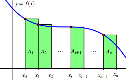
Using Riemann sums to evaluate an integral
Given some $n$, we can therefore approximate $\int_a^b f(x)dx$ withRiemann sums error
How can we estimate the error we are making as function of $n$? Within each interval $[a+kh,a+(k+1)h]$, the worst that can happen is that $f$ changes with constant rate of change equalto the maximum value of the derivative in that interval. In fact, to keep formulae simpler,
we take the max of $f'(x)$ over the whole interval $[a,b]$. We assume $f(x)$ smooth, so its derivative is continuous and therefore $M=\max_{[a,b]}|f'(x)|$ exists for sure.
Riemann sums error
Hence, the largest difference betweenthe value of $f(x)$ at
is $Mh$. In turn, since the length of $[a+kh,a+(k+1)h]$ is $h$, the highest possible error in the estimate of the integral in that interval is the area $\frac{1}{2}Mh^2$ of the triangle with base $h$ and height $Mh$. Since we have $n=\frac{b-a}{h}$ summands, a bound to the total error is
Convergence Speed
Newton-Cotes Quadrature
Of course we'd be happier with a faster convergence than linear. Interpolation is a way to get this goal:we approximate $f(x)$ with some polynomial $p_n(x)$, so that $$ \int_a^bf(x)dx\simeq\int_a^bp_n(x)dx $$ A quadrature rule based on an interpolant polynomial $p_n$ at $n+1$ equally spaced points is called a Newton-Cotes formula of order $n$.
Estimate of error
Remember that, when interpolation points are equidistant, $$ \max_{x\in[a,b]}|f(x)-p(x)|\leq\frac{\displaystyle\max_{x\in[a,b]}\left|\prod_{i=1}^{n+1}(x-x_i)\right|}{(n+1)!} \max_{x\in[a,b]}|f^{(n+1)}(x)|. $$ Similarly, the bound on the integral is given byNewton-Cotes Drawbacks
Since $h=(b-a)/n$, it seems that, by making $n$ large,we have good chances to make the error as small as we please. Unfortunately it is not so, due to the Runge phenomenon. An easy fix for this problem is to keep $n$ low and improve accuracy by dividing, as in case of the Riemann sum, the domain in small intervals and then summing up all contributions. This way, all single summands will have a precision given by the formula in the slide above. Since the number of summands is $N=\frac{b-a}{h}$,
the error in the computation of the integral goes as $h$ to
namely a method built over an interpolation of order
will converge with an error of order
Midpoint rule ($n=0$)
Take $x_0=\frac{a+b}{2}$. Then $w_0=\displaystyle\int_a^bdx=b-a$ and
Local Error in Midpoint rule
Global Error in Midpoint rule
To make this rules useful, the trick is always the same: we divide $[a,b]$ into $n=(b-a)/h$ segments $[x_i,x_{i+1}]$ of length $h$. On each segment, the error bound is
Convergence Speed
Trapezoidal rule ($n=1$)
Take $x_0=a$ and $x_1=b$. Then
Trapezoidal rule error
From the Newton-Cotes error formula, the local error isConvergence Speed
Simpson rule ($n=2$)
Take $x_0=a$, $x_1=(a+b)/2$ and $x_2=b$. ThenSimpson rule error
From the Newton-Cotes error formula (recall that $n$ is even and so we need to use the reminder for $n=4$), the error bound isConvergence Speed
Numerical Methods for ODEs
Initial Value Problems
Existence and uniqueness of smooth solutions
Picard-Lindelof-Cauchy-Lipschitz Theorem
Consider the Initial-Value Ordinary Differential Equation
$$
\dot x = f(t,x)\,,x(t_0)=x_0\,,\;\;t\in\Bbb R,\;x\in\Bbb R^m.
$$
If $f$ is smooth
for all $x\in\Bbb R^m$ and $t\in\Bbb R$,
the ODE system above has a unique solution
defined at all times $t$ close enough to $t_0$.
Example 1
$f(t,x)=x$ is smooth for all $t$ and $x$. Hence, the ODEExample 2
$f(t,x)=x^2$ like in Example 1, is smooth for all $t$ and $x$. Hence, the ODEExample 3
$f(t,x)=\sqrt{x}$ is smooth everywhere (in its domain) except at $x=0$, where $f_x(t,x)=\frac{1}{2\sqrt{x}}$ blows up. Hence uniqueness is not granted there (for existence, continuity is enough). This is why, in this case, there are infinitely many solutions toNumerical Methods
Consider the case when the right hand side depends only on $t$:Explicit Euler Method
This is the simplest numerical method to solve the IVPEuler method $\Longleftrightarrow$ left Riemann sums
When $f$ depends on $t$ only, $$ x_1 = x_0 + hf(t_0), $$ $$ x_2 = x_0 + hf(t_0) + hf(t_0+h), $$ $$ \dots, $$ $$ x_n = x_0 + hf(t_0) + hf(t_0+h) + \dots + hf(t_0+(n-1)h), $$ namelyGlobal error in the Explicit Euler method
When the rhs $f(t,x)$ does not depend on $x$, we know already that the method is of order 1. What to do when it does depend on $x$? In this case, we cannot take the maximum of $|f(t,x)|$ because there is no way to know the range of $x(t)$! We need a new argument. Let $x(t)$ be the exact solution of the ODE and setAn implementation of the Explicit Euler method
Convergence speed of the Explicit Euler method
Other explicit methods
As mentioned before, all methods for numerical quadraturedo translate into methods for numerical solution of ODEs. As an example, here we show only what happens
in case of the trapezoidal method. If $f(t,x)$ depended on $t$ only,
the "local" version of the method would be $x_{n+1}=x_n+\frac{h}{2}\left(f(t_n)+f(t_{n+1})\right)$ Naively, one would want to use $x_{n+1}=x_n+\frac{h}{2}\left(f(t_n,x_n)+f(t_{n+1},x_{n+1})\right)$ but we now we have $x_{n+1}$ on both sides!
Heun Method
A way to overcome the problem aboveis evaluating a first time $x_{n+1}$ using Euler`s method
and use that value into the trapezoidal algorithm. The method obtained this way is an example of "two steps method",
since two steps are needed to evaluate $x_{n+1}$,
and it is called Heun method:
$\hat x_{n+1} = x_n + h f(t_n,x_n)$ $x_{n+1} = x_n + \frac{h}{2}(f(t_n,x_n)+f(t_{n+1},$ $\hat x_{n+1}$ $))$
Stiff ODEs and the Implicit Euler Method
The explicit Euler method and, in general,methods that come from generalization of Newton-Cotes methods,
don`t do well with a type of ODEs called
of the qualitative behavior of the exact solution of the ODE:
follow the same qualitative behavior of the exact solution. See in the next slide a concrete example
of had badly the algorithm can behave.
$\dot x = -15x$, Explicit Euler
Implicit Euler method
This problem disappears if, at the step $n$, we evaluate the right hand side at $x_{n+1}$ rather than $x_n$:The word implicit referes to the fact that the relation above
defines $x_{n+1}$ only implicitly:
an equation must be solved, usually numerically, to get its value. Although clearly much less trivial than its explicit counterpart,
the implicit version has a great advantage:
it behaves well with stiff problems!
does converge monotonically to 0, just like the exact solution!