Press ? for presentation controls.
Best viewed in Firefox,
Chrome and
Opera.
Numerical Methods
for ODE
Initial Value Problems
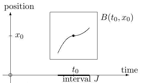
Picard-Lindelof-Cauchy-Lipschitz Theorem
for some $\epsilon>0$.
Example 1
The function $$f(t,x)=x$$ is continuous in $t$ (it doesn't appear!) and uniformly Lipschitz in $x$ (all polynomials are!), so a solution to the IVP $$ \dot x=x\,,\;x(t_0)=x_0 $$ exists and is unique for all $(t_0,x_0)$. Its analytical expression is given by $$x(t)=x_0e^{t-t_0},$$ so individual solutions are defined for all times.Example 2
As before, the function $$f(t,x)=x^2$$ is continuous in $t$ and unif. Lipschitz in $x$, so a solution to $$ \dot x=x^2\,,\;x(t_0)=x_0 $$ exists and is unique for all $(t_0,x_0)$. On the other size, it grows too fast and, because of this, each individual solution blows up in finite time: $$ x(t) = \frac{x_0}{1-x_0(t-t_0)}\hbox{ diverges for } t\to t_0+\frac{1}{x_0}. $$Example 3
The function $$f(t,x)=\sqrt{x}\,,\;x\geq0$$ is continuous in $t$ (it doesn't appear!) but not uniformly Lipschitz in $x$, so the uniqueness of the solution to the IVP $$ \dot x=\sqrt{x}\,,\;x(t_0)=x_0\geq0 $$ is not granted (for existence, continuity is enough). In fact, in this case there are infinitely many solutions for every initial condition $(t_0,x_0)$ with $x_0\geq0$. For instance, $x_1(t)=t^2/4$ and $x_2(t)=0$ pass both through the origin at $t=0$ and both solve the ODE above.The Explicit Euler Method
This is the simplest numerical method for solving ODEs IVP.It is just a re-writing of the definition of derivative:
$$ x'(t) = \frac{x(t+h)-x(t)}{h}+O(h)\,, $$ so that
Since $$ x_{n+1} - x(t_{n+1}) = O(h^2) $$
we say that this method is local order 2.
The number of steps to pass from a time $t_0$ to $t_1$
increases as $1/h$ for $h\to0$
and so the global
order of convergence is 1
[since $h\cdot O(h^2)=O(h)$].
Click here for a rigorous proof.
Example 1
In the next two slides we use the Euler methodto evaluate $x(25)$ for the IVP
whose analytical solution (use separation of variables!) is $$ x(t) = e^{-\sin t}\,. $$
Task 1
Plot a log-log graph of the local and global errorof the Explicit Euler method for $t_f=25$ in case of the IVP
whose analytical solution is $$ x(t) = e^{-\sin t}\,. $$
Task 2
Plot a log-log graph of the local and global errorof the Explicit Euler method for $t_f=\pi/4$ and $t_f=1.2927$
in case of the IVP
whose analytical solution is $$ x(t) = \cos t-\sin t. $$
Task 3
Plot a log-log graph of the local and global errorof the Explicit Euler method for $t_f=1$ and $t_f=0.5$
in case of the IVP
whose analytical solution is $$ x(t) = \sqrt{1-t^2}. $$
Task 4
Print all intermediate values of the Explicit Euler methodto evaluate $x(2)$ in case of the IVP
whose analytical solution is $$ x(t) = \frac{5}{t}. $$ See if you can spot a funny patter in the numerical evolution of the solution by trying several different values of $h$.
Stability
A numerical method is stable if it does not diverge when the exact solution does not diverge.Apply the Explicit Euler method to the linear problem $$ \dot x = Kx, x(t_0)=x_0. $$ The method basic step for this equation is $$ x_{n+1} = x_n + h M x_n = (1+hM)x_n $$ so that $$ x_{n} = (1+hM)^n x_0. $$
is stable only when $h$ is small enough to grant that $$ |1+hM|<1. $$
Stiff Systems
ODEs whose solution changes very rapidly are approximatedvery poorly, even at a qualitative level, by the Explicit Euler method
unless $h$ is taken very small.
Consider for instance the IVP
whose analytical solution is $$ x(t) = e^{-15t}\,. $$
Implicit Euler Method
Another way to write the def of derivative is$$ x'(t+h) = \frac{x(t+h)-x(t)}{h}+O(h), $$
from which we get that
This method is again of local order 2 but the value of $x_{n+1}$ is now given only implicitly and in general must be found numerically, e.g. with the Newton method.
As in the explicit case, the global order of convergence is 1. The reason why it can be convenient using this more complicated method rather than the explicit one is that, as we are going to see below, this method works also for stiff equations, when the explicit one fails.
Task 1
Plot a log-log graph of the local and global errorof the Implicit Euler method for $t_f=25$ in case of the IVP
whose analytical solution is $$ x(t) = e^{-\sin t}\,. $$
Task 2
Plot a log-log graph of the local and global errorof the Implicit Euler method for $t_f=\pi/4$ and $t_f=1.2927$
in case of the IVP
whose analytical solution is $$ x(t) = \cos t-\sin t. $$
Task 3
Plot a log-log graph of the local and global errorof the Implicit Euler method for $t_f=1$ and $t_f=0.5$
in case of the IVP
whose analytical solution is $$ x(t) = \sqrt{1-t^2}. $$
Task 4
Print all intermediate values of the Implicit Euler methodto evaluate $x(2)$ in case of the IVP
whose analytical solution is $$ x(t) = \frac{5}{t}. $$ See if you can find a reason for what you see.
Stability
Apply the Implicit Euler method to the linear problem $$ \dot x = Kx, x(t_0)=x_0. $$ The method basic step for this equation is $$ x_{n+1} = \frac{x_n}{1 - h M} $$ so that $$ x_{n} = \frac{x_0}{(1-hM)^n}. $$only when $h$ is small enough to grant that $$ |1-hM|>1. $$
Rounding errors
Numerical methods are usually affected by two sources of error:- a truncation error, depending on the approximations on which the method is based;
- a round-off error, due to the use of floating-point arithmetic.
We analyize below the round-off error in the Explicit Euler method and show a way to keep it at bay.
Round-off errors upper bound
The recursive step of the Euler method is given by $$ x_{n+1} = x_n + h f(t_n,x_n). $$ Recall that, in a sum, the absolute errors sum up.
Since $h$ is usually quite small with respect to $x_n$,
the round-off absolute error in evaluating $x_{n+1}$ is just the error on $x_n$,
and therefore is of the order of
$$
|x_n|\epsilon_m\,,
$$
where $\epsilon_m$ is the 'epsilon-machine' value.
Global error of Euler explicit method
Consider, by simplicity, a case when the $x_n$ are all of the same order of magnitude. Then the round-off error will contribute to the global error of the Euler explicit method by an amount of the order $$ \frac{C}{h}\,, $$ since the number of steps of the method is proportional to $1/h$ and, in the worst case scenario, the errors will all have the same sign.Hence, an upper bound for the global error of the Explicit Euler method has the following expression: $$ e(h) = \frac{C}{h}+C'h\,. $$
Global error of Euler explicit method
We expect therefore the following picture: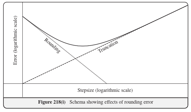
Global error of Euler explicit method
Let's test this prediction on the evaluation of $x(5)$ forCompensated Summation
The problem of accumulation of round-off errors in summations with a large number of summands can be greatly reduced by using the Kahan summation algorithm, also known as compensated summation.
In this method, in order to sum $n$ elements of the array $X = [x(1),\dots,x(n)]$,
we use the following algorithm:
		s=0; e=0;
		for i = 1:n
		    temp = s
		    y = x(i) + e
		    s = temp + y
		    e = (temp-s) + y
		end
Example
Use the compensated sum algorithm to sum the components of $$ X = [10.0,0.23,0.44]. $$ in the naif way and in the compensated method wayin a 3-digits decimal floating-point system.
The exact sum is $10.67$, that approximates to $10.7$
after dropping the 4-th digit.
In the naif summations following the index order, though,
we do not get the correct result:
		s = x(1) + x(2)  = 10.0 + 0.23 = 10.2
		s = s + x(3)  = 10.2 + 0.44 = 10.64 = 10.6
Example
Using the compensated algorithm:temp = s = 0 y = x(1) + e = 10.0 + 0 s = temp + y = 0 + 10.0 = 10.0 e = (temp - s) + y = (0-10.0) + 10.0 = 0 temp = s = 10.0 y = x(2) + e = 0.23 + 0 = 0.23 s = temp + y = 10.0 + 0.23 = 10.2 e = (temp-s) + y = (10.0-10.2) + 0.23 = -0.2 + 0.23 = 0.03 temp = s = 10.2 y = x(3) + e = 0.44 + 0.03 = 0.47 s = temp + y = 10.2 + 0.47 = 10.67 = 10.7 e = (temp-s) + y = (10.2-10.7) + 0.47 = -0.03In short, in the variable $e$ is kept the quantity that is discarded in the sum and then this quantity is added to the new summand.
Euler methods for ODEs in $\mathbb R^n$
and Geometric Integrators

Euler methods in $\mathbb R^n$
A ODE in $\mathbb R^n$ writes as $$ {\mathbf x}(t) = {\mathbf v}({\mathbf x}(t)),\;{\mathbf x}(t_0) = {\mathbf x}_0 , $$ where ${\mathbf x}$ is a point in $\mathbb R^n$ and ${\mathbf v}:\mathbb R^n\to T\mathbb R^n\simeq\mathbb R^n\times\mathbb R^n$ is a vector field. The corresponding recursive step of the explicit Euler method is $$ {\mathbf x}_{n+1} = {\mathbf x}_n + h {\mathbf v}({\mathbf x}_n), $$ the one of the implicit method is $$ {\mathbf x}_{n+1} = {\mathbf x}_n + h {\mathbf v}({\mathbf x}_{n+1}). $$A planar example: the physical pendulum.
Consider $$ \begin{cases} \dot x(t) = y(t),&x(0)=1\cr \dot y(t) = -\sin(x(t)),&y(0)=0\cr \end{cases} $$ and notice that this system is equivalent to the 2nd order ODE $$ \ddot x(t) = -\sin(x(t)),\;x(0)=1,\;\dot x(0)=0 $$ which is the Newtonian equation of motion on $\mathbb R$ of a pointof unitary mass under a force field $F(x)=-\sin(x)$. In particular, there is a conserved quantity: $E(x,y) = \frac{y^2}{2}+1-cos(x)$.
Explicit Euler step
$$ \begin{cases} x_{n+1} = x_n + h y_n\cr y_{n+1} = y_n -h\sin x_n\cr \end{cases} $$Implicit Euler step
$$ \begin{cases} x_{n+1} = x_n + h y_{n+1}\cr y_{n+1} = y_n -h \sin x_{n+1}\cr \end{cases} $$Symplectic Euler step
$$ \begin{cases} x_{n+1} = x_n + h y_{n+1}\cr y_{n+1} = y_n -h \sin x_{n}\cr \end{cases} $$ or $$ \begin{cases} x_{n+1} = x_n + h y_{n}\cr y_{n+1} = y_n -h \sin x_{n+1}\cr \end{cases} $$Runge-Kutta Methods

Taylor series
In principle one could use Taylor expansion beyond first order in order to find new numerical ODE methods. For instance, $$ x''(t) = \frac{d\phantom{t}}{dt}f(t,x(t)) = f_t(t,x(t))+f_x(t,x(t))f(t,x(t)) $$ so one could use $$ x_{n+1} = x_n + h f(t_n,x_n) + \frac{h^2}{2}\left(f_t(t_n,x_n)+f_x(t_n,x_n)f(t_n,x_n)\right) $$ as a method with global error of order 2.Numerical Quadrature
An alternate approach, due to Runge, comes from the observation that, when the r.h.s. of $\dot x=f(t,x)$ does not depend on $x$, the solution of the IVP $x(t_0)=x_0$ writes as $$ x(t)=x_0+\int\limits_{t_0}^t f(t)dt $$ and therefore it can be approximated using the same techniques developed for the numerical quadrature.Example: Explicit Euler method
Consider the left Riemann sum rule: $$ \int\limits_{t_0}^t f(t)dt\simeq\sum_{i=0}^{N-1} f(t_i)h. $$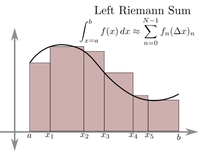
Example: Implicit Euler method
Consider now the right Riemann sum rule: $$ \int\limits_{t_0}^t f(t)dt\simeq\sum_{i=1}^{N} f(t_i)h. $$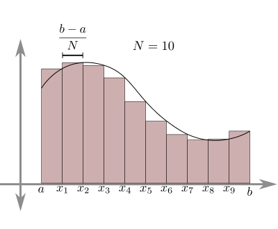
Example: The midpoint method
Consider the midpoint rule $\displaystyle\int\limits_{t_0}^t f(t)dt \simeq \sum_{i=0}^{N-1} f\left(\frac{t_i+t_{i+1}}{2}\right)h$.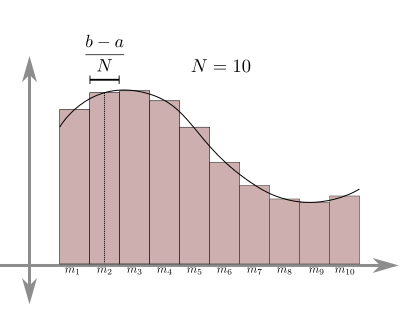
Example: the Heun (trapezoidal) method
The trapezoidal rule gives $ \displaystyle\int\limits_{t_0}^t f(t)dt \simeq \sum_{i=0}^{N-1} \frac{f(t_i)+f(t_{i+1})}{2}h. $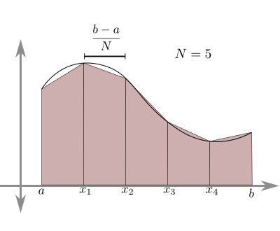
Order of local error
All methods above fit the following scheme: $$ x_{n+1} = x_{n} +h(b_1k_1+b_2k_2), $$ where $$ k_1 = f(t_n,x_n) $$ and $$ k_2=f(t_n+ch,x_n+hak_1). $$ Midpoint method: $b_1=0, b_2=1, c=1/2, a=1/2$ Heun method: $b_1=1/2, b_2=1/2, c=1, a=1$Task 1
Show with Taylor expansion that the choices above make the local error go to zero with $O(h^3)$. You will see that asking all terms of order less than $h^3$amounts to the following conditions: $$ b_1+b_2=1,\;2cb_2=1,\;2ab_2=1. $$
Runge-Kutta methods
Runge and Kutta considered the generalization of this construction: $$ x_{n+1} = x_n + h \sum_{i=1}^s b_i k_i, $$ where $$ k_i = f(t_n+c_ih,x_n+h\sum_{j=1}^s a_{ij} k_j), $$ Explicit RK methods have $a_{ij}$ for $j\geq i$.Butcher Tableau
Traditionally, all these coefficients are arrangedinto a Butcher Tableau:
 Often it is also assumed that $\sum_{j=1}^sa_{ij}=c_i$.
RK4
The most popular RK method is the following: $$ \begin{cases} \displaystyle x_{n+1} = x_n+h\frac{k_1+2k_2+2k_3+k_4}{6}\cr k_1 = f(t_n,x_n)\cr k_2 = f(t_n+\frac{h}{2},x_n+\frac{h}{2}k_1)\cr k_3 = f(t_n+\frac{h}{2},x_n+\frac{h}{2}k_2)\cr k_4 = f(t_n+h,x_n+hk_3)\cr \end{cases} $$- The local error of RK4 is $O(h^5)$.
- Four evaluations of $f$ are needed at every step.
- When $f$ does not depend on $x$, this is the Simpson rule.
Variable Step Size
When the r.h.s. of an ODE changes wildly in some parameter window, a fix step-size is not optimal since either it gives a very rough approximation of the solution(if the step size is chosen too large
with respect to the fluctuations of the function) or it requires an unnecessarily large time to compute
(if it is chosen small enough). In these cases, it is better to implement an algorithm
able to modify the step size
according to the point of the phase space where the solution is.
so that at every step $t_n\to t_{n+1}=t_n+h$,
we have two outcomes $x_{n+1,1}$ and $x_{n+1,2}$.
Notice that, in order to be efficient, we choose the methods so that all evaluations of $f$ for the first will also be used for the second.
Second, we fix a tolerance parameter $\epsilon>0$.
Algorithm:- Evaluate the "euristic" error $e_n = |x_{n+1,1}-x_{n+1,2}$|;
- If $e_n<\epsilon\cdot h$, accept the current $h$ and set $x_{n+1} = x_{n+1,2}$ or to some better approximation (depending on the case, see the example below);
- Otherwise, decrease $h$ through some function of $e_n$ and start again from $t_n$.
A Toy Example: Adaptive Euler
We follow here a nice toy model by Joel Feldman.As first of the two methods, we use the explicit Euler method, namely $$ x_{n+1,1} = x_n + h f(t_n,x_n). $$ Remember that the local error of explicit Euler is $$ \ell_n = K h^2 + O(h^3), $$ or, in other words, $$ x(t_n+h) = x_{n+1,1} + K h^2 + O(h^3), $$ where $x(t)$ is the solution of $x'=f(t,x)$ with $x(t_n)=x_n$.
A Toy Example: Adaptive Euler
As the second method, we use two stepsof the explicit Euler method with half step size, namely $$ x_{n+1,2} = x_n + \frac{h}{2} f(t_n,x_n) + \frac{h}{2} f(t_n+\frac{h}{2},x_n+\frac{h}{2}f(t_n,x_n)). $$ In this case, the local error is $$ \ell_n = K \left[\frac{h}{2}\right]^2 + O(h^3) + K \left[\frac{h}{2}\right]^2 + O(h^3) = K\frac{h^2}{2}+O(h^3). $$
A Toy Example: Adaptive Euler
Hence $$ e_n = |x_{n+1,1}-x_{n+1,2}| = K\frac{h^2}{2}+O(h^3), $$ namely this difference tells us precisely the rate of change of the error close to $(t_n,x_n)$: $$ \frac{e_n}{h} \simeq \frac{Kh}{2}. $$A Toy Example: Adaptive Euler
If $e_n<\epsilon\cdot h$, we accept $h$ and set $$ x_{n+1} = 2x_{n+1,2}-x_{n+1,1}. $$ Notice indeed that $$ x(t_n+h) = 2x_{n+1,2}-x_{n+1,1} + O(h^3) $$ because the 2nd order terms cancel out!A Toy Example: Adaptive Euler
If, instead, $e_n>\epsilon\cdot h$, then we chose a new step size $h'$ so that $$ \frac{K}{2}h'<\epsilon, $$ e.g. $h'=0.9\epsilon h^2/e_n$, and we repeat the process. Finally, at every step we start with $$ h_{n+1} = 0.9\epsilon \frac{h_n^2}{e_n} $$A Toy Example: Adaptive Euler
In the next slide we present an implementation of this algorithm to solve our main ODE example: $$ x' = -x\cos t,\;x(0)=1 $$ We plot the solution for $0\leq t\leq 25$.RK34
An example closer to real-life methods comes from the RK34 method, namely an "embedded pair" of RK methods of order 3 and 4: $$ \begin{cases} k_1 = f(t_n,x_n)\cr k_2 = f(t_n+\frac{h}{2},x_n+\frac{h}{2}k_1)\cr k_3 = f(t_n+\frac{h}{2},x_n+\frac{h}{2}k_2)\cr k'_3= f(t_n+h,x_n-hk_1+2hk_2)\cr k_4 = f(t_n+h,x_n+hk_3)\cr x_{n+1} = x_n+h\frac{k_1+2k_2+2k_3+k_4}{6}\cr x'_{n+1} = x_n+h\frac{k_1+4k_2+k'_3}{6}\cr \end{cases} $$BVP problems
Definition
We will consider here only one of the simplest cases of Boundary Value Problems (BVPs), namely the ODE $$ x''=f(t,x,x')\,,\;x(t_b)=x_b\,,\;x(t_e)=x_e. $$ A solution to this equation is any $C^2$ map $\gamma:\Bbb R\to\Bbb R$ such that $\gamma''(t) = f(t,\gamma(t),\gamma'(t))$ for every $t\in[t_b,t_e]$ and, moreover, $\gamma(t_b)=x_b$ and $\gamma(t_e)=x_e$. The terminology BVP comes from the fact that the problem fixesthe values of the solution at the boundary points
of the set on which is defined the independent variable $t$.
Existence and Uniqueness
Given the BVP problem $$ x''=f(t,x,x')\,,\;x(t_b)=x_b\,,\;x(t_e)=x_e, $$ does a unique solution exists for every choice of $t_0,t_1,x_0,x_1$? Simple examples show that this is not the case (see below).Example 1
Consider the BVP problem $$ x''=-x\,,\;x(0)=0\,,\;x(\pi)=0. $$ The general solution of $x''=-x$ is $$ x(t)=A\cos(t)+B\sin(t). $$ Since $x(0)=0$, it must be $A=0$ and so, since $\sin(\pi)=0$,every function $x(t)=B\sin(t)$ solves the problem,
namely this problem has infinitely many solutions!
Example 2
Now consider instead $$ x''=-x\,,\;x(0)=0\,,\;x(\pi/2)=0. $$ Again, from $x(0)=0$ we get that $x(t)=B\sin(t)$but then $x(\pi/2) = B\sin(\pi/2)=B$
and so there is in this case a unique solution: $$ x(t)=0. $$
Example 3
Finally consider $$ x''=-x\,,\;x(0)=0\,,\;x(\pi)=1. $$ We already notice that if $x(0)=0$ then $x(\pi)=0$,so in this case there is no solution to this problem.
Application 1: Geodesics
Given two points $p$, $q$ on a Riemannian manifold $M^n$with metric tensor $g=g_{\mu\nu}dx^\mu dx^\nu$, $1\leq\mu,\nu\leq n$,
the shortest path joining $p$ with $q$
is the segment of geodesics with those endpoints,
namely the image of the solution of the BVP problem $$ \ddot x^\lambda + \Gamma^\lambda_{\mu\nu}(x)\dot x^\mu\dot x^\nu = 0,\,x(0)=p,\,x(1)=q. $$ The $\Gamma^\lambda_{\mu\nu}(x)$ are called Christoffel symbols and are given by $$ \Gamma^\lambda_{\mu\nu} = \frac{1}{2}g^{\lambda\gamma}\left(\partial_\mu g_{\gamma\nu} + \partial_\nu g_{\gamma\mu} + \partial_\gamma g_{\mu\nu}\right). $$ See the examples below for more details on this formula.
Remark 1
Note that the $\Gamma^\lambda_{\mu\nu}(x)$ are not the components of a tensorbut rather of an affine connection. For instance, it is always possible to choose coordinates
such that all $\Gamma^\lambda_{\mu\nu}(x)$ are zero at a given point. This would be impossible for a non-zero tensor because,
if a tensor is zero at a point in a coordinate system,
then it would be equal to zero in any other system.
Remark 2
If $\gamma_0(t)$ is a solution of this problem,the curve $\gamma(t) = \gamma_0(\frac{t-t_b}{t_e-t_b})$ solves the BVP $$ \ddot x^\lambda + \Gamma^\lambda_{\mu\nu}(x)\dot x^\mu\dot x^\nu = 0,\,x(t_b)=p,\,x(t_e)=q $$ for any $t_b\neq t_e$. This correspond to walking over the same curve
with a different (constant!) velocity.
Example: Geodesics on the Euclidean plane
The Euclidean metric on the plane is the $(0,2)$ tensor field $g=dx^2+dy^2$. The corresponding matrix is $$ \left(g_{\mu\nu}\right) = \begin{pmatrix}1&0\cr 0&1\cr\end{pmatrix}. $$ The inverse matrix is the $(2,0)$ tensor field $$ \left(g^{\mu\nu}\right) = \begin{pmatrix}1&0\cr 0&1\cr\end{pmatrix}. $$Example: Geodesics on the plane
Since the $\Gamma^\lambda_{\mu\nu}$ are defined in terms of the derivatives of the $g_{\mu\nu}$,all Euclidean Christoffel symbols are identically zero
and the geodesic equations are given by the system $$ \begin{cases} \ddot x=0\cr \ddot y=0\cr \end{cases} $$ The general solution of the system is clearly $$ \begin{cases} x(t)=at+b\cr y(t)=ct+d\cr \end{cases} $$ and so the unique geodesic segment between any two points $(x_0,y_0)$ and $(x_1,y_1)$ is the segment of straight line between them.
Example: Geodesics on the sphere
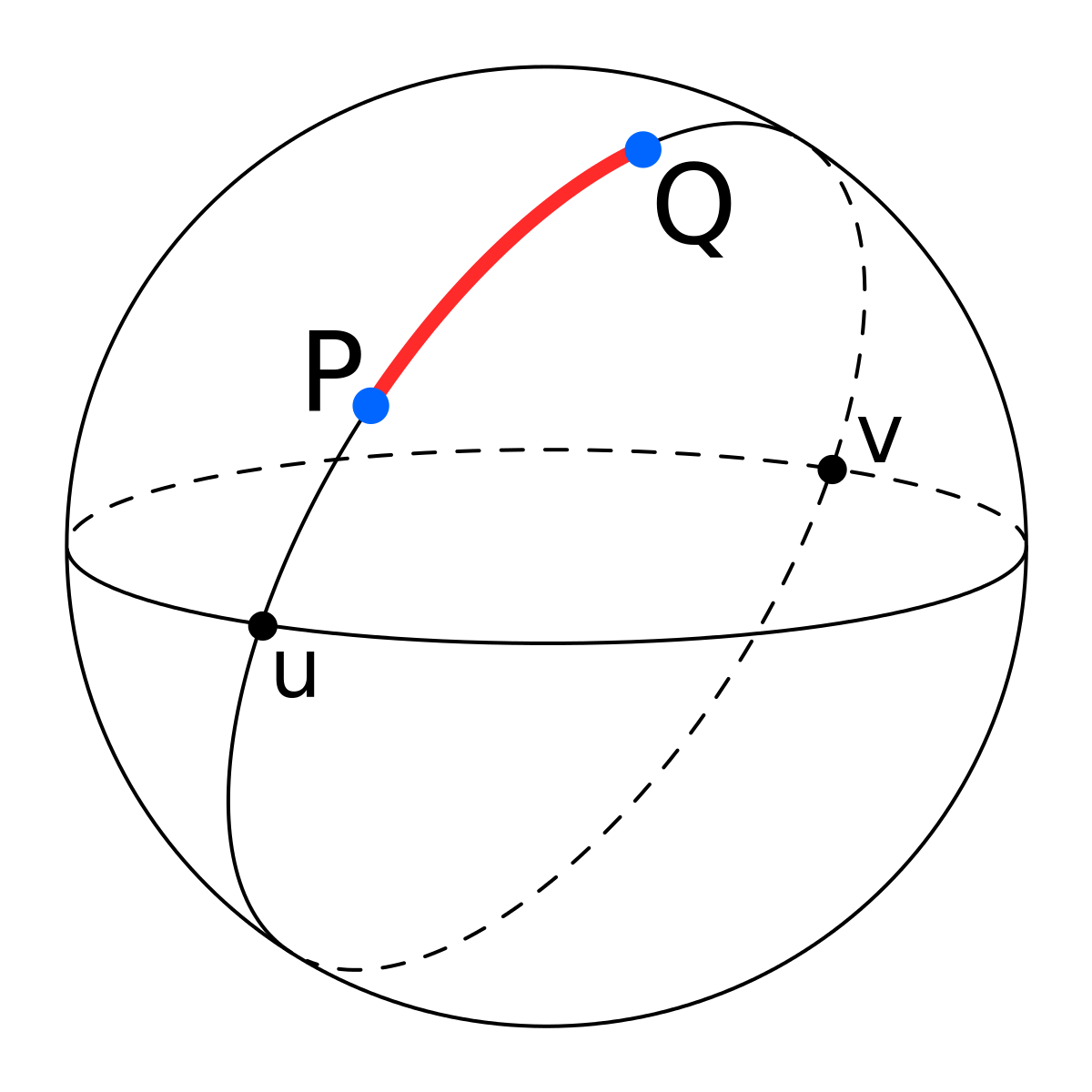
Given any two non-antipodal points $p,q$ on $\Bbb S^2$, there is a unique segment of geodesic between them, given by the shortest segment of the great circle passing through $p$ and $q$ (see figure below). (Recall that, through any two non-antipodal points $p,q$, passes always a single great circle, given
by the intersection of the sphere with a plane passing through its center and the points $p,q$.)
The chart
Let us prove this statement using the geodesics equations. Because of the symmetry, it is enough to consider what happens to the geodesics coming out from the south pole. About this point, we will consider the chart given by the stereographic projection. In concrete, we consider the sphere of radius 1 centered at the origin and, for any point
$(x,y,z)$ different from the north pole,
In concrete, we consider the sphere of radius 1 centered at the origin and, for any point
$(x,y,z)$ different from the north pole,we use coordinates $(X,Y)=(\frac{x}{1-z},\frac{y}{1-z})$.
The metric in coordinates
Given a point with stereographic coordinates $(X,Y)$,the corresponding point on the sphere is $\left(\frac{2X}{1+X^2+Y^2},\frac{2Y}{1+X^2+Y^2},\frac{-1+X^2+Y^2}{\phantom{-}1+X^2+Y^2}\right)$. (Just solve the system $x=X(1-z), y=Y(1-z),x^2+y^2+z^2=1$) Hence, the metric on the sphere in these coordinates is given by $$ g_{\Bbb S^2}(X,Y) = dx^2(X,Y)+dy^2(X,Y)+dz^2(X,Y) $$ $$ = $$ $$ \frac{4}{(1+X^2+Y^2)^2}\left(dX^2+dY^2\right). $$
The metric's matrix
In matrix notation, this means that $$ \left(g_{\mu\nu}\right) = \frac{4}{(1+X^2+Y^2)^2}\begin{pmatrix}1&0\cr 0&1\cr\end{pmatrix}, $$ whose inverse is $$ \left(g^{\mu\nu}\right) = \frac{(1+X^2+Y^2)^2}{4}\begin{pmatrix}1&0\cr 0&1\cr\end{pmatrix}. $$Christoffel symbols
A direct calculation from the definition shows thatthe corresponding Christoffel symbols are $$ \Gamma^X_{XX} = \Gamma^Y_{XY} = \Gamma^Y_{YX} = -\Gamma^Y_{XX} = -\frac{2X}{1+X^2+Y^2} $$ and $$ \Gamma^Y_{YY} = \Gamma^X_{XY} = \Gamma^X_{YX} =-\Gamma^X_{YY} = -\frac{2Y}{1+X^2+Y^2} $$ Notice that, in these coordinates, all Christoffel symbols
are equal to zero at the south pole ($X=Y=0$).
Geodesics Equations
The geodesics equations in these coordinates therefore are: $$ \begin{cases} (1+X^2+Y^2)\ddot X-2X\dot X^2+2Y\dot Y^2-4Y\dot X\dot Y=0\cr (1+X^2+Y^2)\ddot Y+2Y\dot X^2-2X\dot Y^2-4X\dot X\dot Y=0\cr \end{cases} $$ Rather than looking for a general solution for this equation, we show that the equations of a motion with constant angular speedon a great circle does solve it.
Existence of BVP solutions
Notice first that we can always rotate the sphere so that a point moving with const. angular speed on a great circle has parametric eq. $$ t\mapsto (\sin t,0,\cos t). $$ In $(X,Y)$ coordinates, this writes $\displaystyle t\mapsto\left(\frac{\sin t}{1-\cos t},0\right)$.The geodesics equations with $Y(t)=0$ reduce to $$ (1+X^2)\ddot X-2X\dot X^2=0 $$ and a direct check shows that the function $X(t) = \sin t/(1-\cos t)$ does solve this equation.
The parameter is important!
Notice that the curve $t\mapsto(t,0)$ does not solve the geodesics equations although its image is a great circle too! This is due to the fact that its angular speed is not constant, namely the parameter is not proportionalto the curve's arclength parameter of that curve.
Uniqueness of BVP solutions
Why are these solutions unique? There are several geometric elementary arguments (e.g. see this discussion).Here we rather use the following fact. Denote by $T_S\Bbb S^2\simeq\Bbb R^2$ the tangent plane to the sphere
at the south pole and consider the exponential map $$ T_S\Bbb S^2\to \Bbb S^2 $$ that associates to an initial speed $v$ the point reached at $t=1$ by the geodesic line leaving the south pole at $t=0$ with speed $v$.
Jacobian of the Exponential Map
The Jacobian of the exponential map at $v=0$ is the identity,so that this map is a diffeomorphism for small enough $v$. Indeed, call $(X_v(t),Y_v(t))$ the sol. to the geodesic equations passing at $t=0$ through the south pole with vel. $v=(v_X,v_Y)$.
For $v$ small enough, the velocity keeps being very small up to $t=1$, namely in linear approximation the geodesics equations reduces to $$ \ddot X = \ddot Y = 0. $$ The solution is therefore $$ X_v(t) = v_X\cdot t+O(v^2),\,Y_v(t) = v_Y\cdot t+O(v^2) $$ Hence the Jac. of $(v_X,v_Y)\mapsto(X_v(1),Y_v(1))$ is the identity.
Uniqueness of BVP solutions
Due to the implicit function theorem, the geodesic between the south pole and any point close enough to it is unique and it is an arc of great circle parametrized so that the angular velocity is constant. This means that all geodesics coming out from every point are great circles. The uniqueness fails when two of such curves meet. In a given stereographich map this never happens, so there is a unique geodesics joining the north pole to any point but the only point not covered by the stereographic chart, namely the north pole. In that last case we know that there is no uniqueness because there are infinitely many great circles joining two antipodal points.Application 2: Sturm-Liouville problems
Every linear 2nd order ODE can be written in the form $$ \frac{d\phantom{x}}{dx}\left[p(x)\frac{dy}{dx}\right]+q(x)y=-\lambda w(x)y. $$ This is called Sturm-Liouville equation. This problem is equivalent to finding the eigenvalues $\lambda$of the infinite-dimensional linear operator $$ \cal L y = \frac{p}{w}y''+ \frac{p'}{w}y'+ \frac{q}{w}y. $$ The existence and behavior of the eigenvalues
depends strongly on the boundary conditions.
Example: Quantum Mechanics
In Quantum Mechanics a particle in $\Bbb R^n$ (or some subset of it) is not represented, like in classical mechanics, by a point in $\Bbb R^n$but rather by a wave function $\psi\in L^2(\Bbb R^n)$,
namely a complex function $\psi:\Bbb R^n\to\Bbb C$ such that $$ \int_\Bbb R^n|\psi(x)|^2d\mu(x)=1, $$ where $\mu$ is the Lebesgue measure. The meaning of $\psi$ is that the probability to find the particle in a region $D\subset \Bbb R^n$ is equal to $ \int_D|\psi(x)|^2d\mu(x). $ Observables (i.e. energy, position, momentum and so on) are replaced by self-adjoint linear operators on $L^2(\Bbb R^n)$ and the result of a measurement of an observable cannot be any number but rather an eigenvalue of the corresponding operator.
Quantum Particle in a 1D box
The Energy operator of a particle in a potential filed $V(x)$ is given by $H=-\frac{d^2\phantom{x}}{dx^2}+V(x)$.In case of a free particle inside a box of side $a$, then it is $H=-\frac{d^2\phantom{x}}{dx^2}$.
Since the particle is bound to stay inside the box, the wave function must be identically zero outside of the box $[0,a]$ and so,
by continuity, it must be zero also at the endpoints.
Hence, the eigenvalues of $H$ are the solutions of the BVP $$ -\psi'' = \lambda\psi,\,\psi(0)=\psi(a)=0. $$ Notice that this is a Sturm-Liouville problem
with $p(x)=1$, $q(x)=0$ and $w(x)=1$.
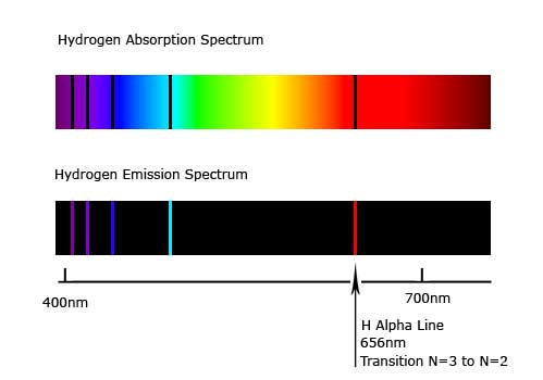
Note that, in particular, there is only a discrete set of possible outcomes of a measurement of the Energy of a particle inside such box. This is a toy model for the spectra of electrons in an atom
(see below the spectra of the hydrogen atom).
Shooting Method
Assuming that there is a solution to $$x''=f(t,x,x')\,,\;x(t_b)=x_b\,,\;x(t_e)=x_e\,,$$ the shooting method's idea is using IVP to find better and better approximations of the value of $x'(t_b)$ that produces a solution $x(t)$ s.t. $x(t_e)=x_e$.

Call $F(v)$ the value at $t=t_e$ of the solution of the IVP $$x''=f(t,x,x')\,,\;x(t_b)=x_b\,,\;x'(t_b)=v\,.$$ This is a function $F:\Bbb R\to\Bbb R$
and the $v$ we are looking for is a solution of the equation $$ F(v) = x_e\,. $$ One can now use numerical methods of equation solving to find $v$. The most well known of these methods is the Newton method.The linear case
A particularly simple case it the linear one. Recall the following theorem: the space of solutions of a linear ODE $$ x' = Ax,\,x(t_b)=x_b,\,x\in\Bbb R^n $$ is itself a linear space. Moreover, the map that sends an initial condition $x_b$ to the corresponding solution is a linear map. In fact, the explicit expression of that map is given by $$ x_b\mapsto x(t) = e^{A(t-t_b)}x_b. $$The linear case
In particular, this means that for linear BVP $$ \ddot x = a(t) \dot x + b(t) x +c(t),\,x(t_b) = x_b,\, x(t_e)=x_e, $$ the function $F(v)$ is itself linear, namely $$ F(v) = \alpha v+\beta. $$ This means that it is enough to solve numerically two IVP in order to solve the BVP. For instance, say that $F(0) = q_0$ and $F(1) = q_1$. Then $\beta = q_0$ and $\alpha = q_1-q_0$, so that the solution to $$ F(v) = x_e \;\;\mbox{ is }\;\; v = \frac{x_e-q_0}{q_1-q_0}. $$Example
Consider our usual IVP $$ \dot x = -x\cos t,\,x(0)=1,\, $$ whose solution is $x(t)=e^{-\sin t}$ and of which we usually evaluate numerically $x(25)$. Since we need a 2nd order ODE, we will rather consider the BVP given by its "first prolongation" $$ \ddot x = -\dot x\cos t+x\sin t,\,x(0)=1,\,x(25)=e^{-\sin 25}. $$ The code in next slide shows how to solve this BVP.Finite Difference Method
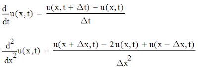
into a (very large) algebraic system of equations. As we already saw, there are several ways to accompish that:
| 1st der. | Forward difference: | $\dot x(t) = \frac{x(t+h)-x(t)}{h} + O(h)$. |
| Backward difference: | $\dot x(t) = \frac{x(t)-x(t-h)}{h} + O(h)$. | |
| Symmetric difference: | $\dot x(t) = \frac{x(t+h)-x(t-h)}{2h} + O(h^2)$. | |
| 2nd der. | Symmetric difference: | $\ddot x(t) = \frac{x(t+h)-2x(t)+x(t-h)}{h^2} + O(h^2)$. |
| 5-points stencil: | $\ddot x(t) = \frac{-x(t+2h)+16x(t+h)-20x(t)+16x(t-h)-x(t+2h)}{12h^2} + O(h^4)$. |
we can approximate the linear infinite-dimensional differentiation operators
$d/dt: x(t)\mapsto \dot x(t)$ and $d^2/dt^2: x(t)\mapsto \ddot x(t)$
with linear finite-dimensional operators.
Below, we focus on sthe case of symmetric ones.
First derivative
$$ \begin{pmatrix}x_0\\ x_1\\ \vdots\\ x_{N-1}\\ x_N\end{pmatrix} \mapsto \begin{pmatrix}x'_1\\ x'_2\\ \vdots\\ x'_{N-2}\\ x'_{N-1}\end{pmatrix} =\frac{1}{2h} \begin{pmatrix}-1&0&1&&\cr &-1&0&1&&\cr &&\ddots&\ddots&\ddots\cr &&&-1&0&1\cr\end{pmatrix} \begin{pmatrix}x_0\\ x_1\\ \vdots\\ x_{N-1}\\ x_N\end{pmatrix} $$ Notice that this is an operator $\Bbb R^{N}\to\Bbb R^{N-2}$.Second derivative
$$ \begin{pmatrix}x_0\\ x_1\\ \vdots\\ x_{N-1}\\ x_N\end{pmatrix} \mapsto \begin{pmatrix}x''_1\\ x''_2\\ \vdots\\ x''_{N-2}\\ x''_{N-1}\end{pmatrix} =\frac{1}{h^2} \begin{pmatrix}1&-2&1&&\cr &1&-2&1&&\cr &&\ddots&\ddots&\ddots\cr &&&1&-2&1\cr\end{pmatrix} \begin{pmatrix}x_0\\ x_1\\ \vdots\\ x_{N-1}\\ x_N\end{pmatrix} $$ Notice that this is an operator $\Bbb R^{N}\to\Bbb R^{N-2}$.The first derivative then becomes the affine map $$ \begin{pmatrix}x'_1\cr x'_2\cr\vdots\cr x'_{N-2}\cr x'_{N-1}\end{pmatrix} =\frac{1}{2h} \begin{pmatrix} 0&1&&\cr -1&0&1&&\cr &\ddots&\ddots&\ddots\cr &&-1&0&1\cr &&&-1&0\cr \end{pmatrix} \begin{pmatrix}x_1\cr x_2\cr\vdots\cr x_{N-2}\cr x_{N-1}\end{pmatrix} + \frac{1}{2h} \begin{pmatrix}-x_b\cr 0\cr \vdots\cr 0\cr x_e\end{pmatrix} $$
Example
Consider again the problem $$ \ddot x = -\dot x\cos t+x\sin t,\,x(0)=1,\,x(25)=e^{-\sin 25}, $$ that we already solved with the shooting method. The python code below uses the finite differences codeto solve the general BVP problem $$ \ddot x = u(t) + v(t) x +w(t) \dot x,\,x(t_b)=x_b,\,x(t_e)=x_e. $$
Application Example: Poincare' map
Fixed points and Periodic solutions of an ODE
Nonlinear ODEs in dimension higher than 1 can have a quite complicated behavior, even when they have a simple expression.E.g., one of the first examples of such systems is the Lorenz system, introduced in 1963 by the mathematician and metereologist Edward Lorenz as a simple model of atmospheric convection. There are two simple elements that provide important information on the global behavior of the ODE solutions:
- the behavior of solutions nearby constant solutions, namely near points that make the r.h.s. of the equation equal to zero;
- the behavior of solutions nearby periodic solutions, namely solutions whose image is a loop.
Poincare' map
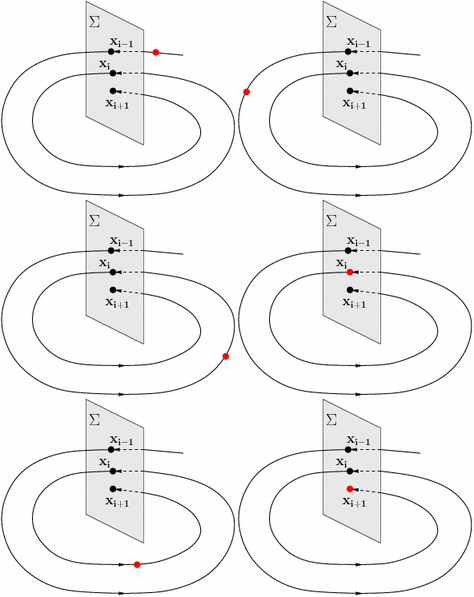
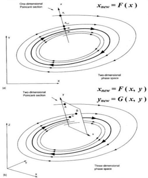
Here we we focus on the second element. Suppose that the ODE admits a periodic solution, namely the image of that solution is a loop.How to study the behavior of trajectories nearby the periodic one? Poincare's idea is the following.
Take a plane $\pi$ transversal to the loop at some point $P_0$. Then, for all points $P$ close enough to $P_0$, take the solution of the ODE with initial condition $P$ and call $f(P)$ its next intersection with $\pi$ from the same side. This defines a function $f$ from some nbhd of $P_0$ into itself that tells a lot about the global behavior of solutions of the ODE.
Poincare' map
Example: Henon-Heiles
Below is an example of Poincare' map in case of the Henon-Heiles system, a 2D mechanical system introduced in 1962 to model the motion of a star around a galactic center.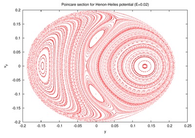
on a 2-torus containing the loop...
Example: Henon-Heiles
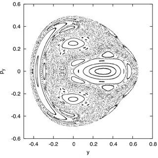
...but for other parameter valuessome orbits behave in a quite different way:
A worked-out example: the Lorenz system
The Lorenz system is the following 3D ODE: $$ \begin{cases} \dot x(t) = 10(x-y)\cr \dot y(t) = \rho x-y-xz\cr \dot z(t) = xy-\frac{8}{3}z\cr \end{cases} $$ We choose $z=\rho-1$ as our Poincare' map plane. In the code below, we use RK4 to integrate the Lorenz systemand visualize the iterations of the Poicare' map. (In order to see a decent resolution picture
you will need to run the code on your machine
since there is a short time bound on the applet running time!)
Poincare' map
Poincare' map
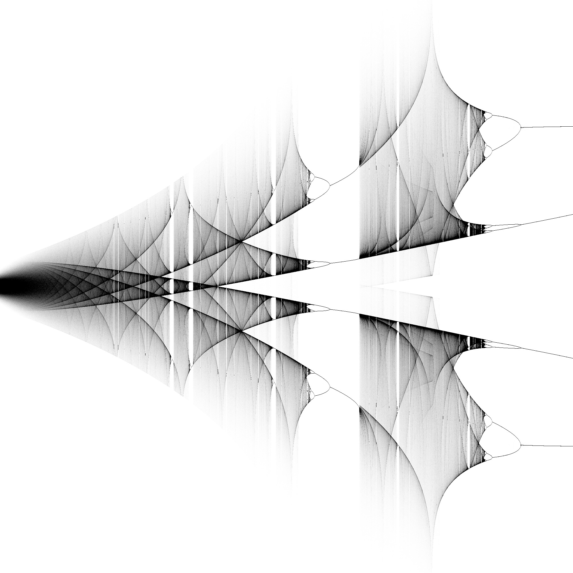
Below is a picture obtained setting $w=h=2000$and $t_f=10000$:
Proofs
Order of the Explicit Euler method
The global error at the $n$-th step is given by $$e_n = x(t_n)-x_n\,,$$ where $x(t)$ is the solution of the IVP problem. Hence $$ e_{n+1} = e_n +h \left(f(t_n,x(t_n))-f(t_n,x_n)\right) + \ell_n\,, $$ where $\ell_n$ is the local error at $(t_n,x_n)$.Since $f$ is Lipschitz in $x$, $$ \left|f(t_n,x(t_n))-f(t_n,x_n)\right|\leq L_n |e_n||x(t_n)-x_n|=L_n|e_n|\,. $$
and local errors over all $1\leq n\leq N$.
Then $$ |e_{n+1}\leq L(1+hL)e_n+\ell\,. $$ Hence $$ |e_{n}|\leq (1+hL)^n)|e_0|+\ell\sum_{k=1}^{n-1}(1+hL)^k. $$
- Neglect round-off error: $e_0=0$;
- Recall that local error is $O(h^2)$: $|\ell|\leq A h^2$ for $A=\frac{1}{2}\sup|x''(t)|$;
- Recall that $\sum_{k=1}^{n-1}q^k=\frac{1-q^n}{1-q}$.
Then: $$ |e_{n}|\leq \frac{h}{2L}(e^{Lt_f}-1)\sup|x''(t)|\,, $$ where $t_f$ is the final time.