Partial
Differential
Equations
Digression:
vectors and covectors
Linear PDEs of 1st order
Definition
A linear PDE of 1st order on a set $\Omega\subset\Bbb R^n$ is an equation of the form $$ X^\alpha(x)\partial_\alpha u(x) + \mu(x) u(x)= v(x)\,, $$ where $v\in C^k(\Omega)$ and $\mu,X^\alpha\in C^\infty(\Omega)$, $\alpha=1,\dots,n$. Note that $X=X^\alpha(x)\partial_\alpha$ is a smooth vector field on $\Omega$ and $Xu$ is the directional derivative of $u$ with respect to $X$. When $\mu=0$, the equation $$ Xu(x) = v(x)\,, $$ is called cohomological equation.Example
The simplest example of this kind of PDE is $$ \partial_x u(x,y) = v(x,y)\,,\;v\in C^{k}(\Omega) $$ whose general solution, close to a point $(x_0,y_0)$, is locally given by $$ u(x,y) = \int\limits_{x_0}^x g(x,y)dx + h(y)\,. $$ Note that, unlike what happens for ODEs, there is no restriction on $h(x)$ (in principle it could belong to $L^1_{loc}(\Omega)$) and so the smoothness of the r.h.d. does not imply any global regularity of $u$ on $\Omega$.Important general properties
The coefficients $(X^1(x),\dots,X^n(x))$ are the components of a vector field on $\Omega$.
The partial differential operator $D=X^\alpha(x)\partial_\alpha$ does not
depend on the coordinate systems. When we change coordinates
$x^\alpha\to x^{\alpha'}(x^\alpha)$ then (chain rule)
$$
\partial_{\alpha'} = \left(\partial_{\alpha'}x^\alpha\right)\partial_\alpha\,,
$$
so that
$$
X^\alpha = X^{\alpha'}\partial_{\alpha'}x^\alpha\,,
$$
that is exactly the change of coordinates rule for a vector.
Important general properties
We can locally trade the zero order term for a second cohomological equation.
When there is a solution to $X\rho=\mu$, the equation
$$
Xu(x) + \mu(x) u(x)= v(x)
$$
is equivalent to the system
$$
\begin{cases}
X\rho(x) = \mu(x)\\
X\left(e^\rho(x) u(x)\right) = e^\rho(x)v(x)
\end{cases}\,,
$$
since $e^\rho(x)>0$ for all $x\in\Omega$.
A solution to $X\rho=\mu$ exists always locally (see the slides below).
PDE/ODE interplay
The solvability of the PDE $X^\alpha\partial_\alpha u=v$ is strictly related with the topology of the integral trajectories of the vector field $X=(X^1,\dots,X^n)$, namely of the solutions of the ODE system $$ \begin{cases} \dot x^1(t) = X^1( x^1(t),\dots,x^n(t))\\ \dots\\ \dot x^n(t) = X^n( x^1(t),\dots,x^n(t))\\ \end{cases} $$ Remark: we can assume WLOG that $X$ is complete, namely that the solutions to the ODE systems above extend to all times.Considered that we are assuming $X$ to be smooth (so that uniqueness is granted), the only obstruction to this would be that solutions reach infinity at a finite time (as it happens, for instance, in case of $\dot x = x^2$).
In case $X$ is not complete, by Godbillon, Dynamical Systems on Surfaces, Prop. 1.19, there is always a positive smooth function $f$ such that $Y=f X$ is complete, so that $Xu=v$ iff $Yu=fv$.
Local Solvability of Linear 1st order PDEs
Assume then that $X$ is complete and let $\Phi^t_X$ be the flow of $X$, namely the 1-parameter group of diffeomorphisms of $\Omega$ into itself such that $$ \frac{d\phantom{t}}{dt}\Phi^t_X(x_0)\bigg|_{t=0} = X(x_0)\,, $$ and let $\Gamma$ be a smooth curve always transversal (i.e. never tangent) to the integral trajectories of $X$. Then the PDE $$ Xu=v\,,\; u|_\Gamma = h $$ has a unique solution on the set $\Phi_X(\Gamma)=\cup_{t\in\Bbb R}\Phi_X^t(\Gamma)\subset\Omega$ given by $$ u(x) = \int_0^t v(\Phi^\tau_X(x_0))d\tau + h(x_0) $$ where $t$ is the (unique!) solution of the equation $\Phi^{-t}_X(x)\in\Gamma$ and $x_0=\Phi^{-t}_X(x)$.Proof
By definition $Xu(x)$ is the derivative of the restriction of $u$ to any curve passing through $x$ with velocity vector $X(x)$ so, in particular, $$ Xu(x) = \frac{d\phantom{t}}{dt}u(\Phi^t_X(x))\bigg|_{t=0}\,. $$ Let $x=\Phi^{\bar t}_X(x_0)$, $x_0\in\Gamma$. Since the $\Phi^t_X$ are a group with respect to $t$, namely $\Phi^t_X\Phi^s_X=\Phi^{t+s}_X$, then $$ u(\Phi^t_X(x)) = u(\Phi^t_X(\Phi^{\bar t}_X(x_0))) = u(\Phi^{t+\bar t}_X(x_0)) $$ and so $$ Xu(x) = \frac{d\phantom{t}}{dt}u(\Phi^{t+\bar t}_X(x_0))\bigg|_{t=0} = \frac{d\phantom{t}}{dt}\left[\int_0^{t+\bar t} v(\Phi^\tau_X(x_0))d\tau + h(x_0)\right]_{t=0} = $$ $$ = v(\Phi^{\bar t}_X(x_0)) = v(x)\,. $$ Uniqueness: prove it!Regularity of solutions
Assume that $v\in C^k(\Omega)$ and $h\in C^k(\Gamma)$. Then the local solution defined above
lies in $C^k(\Phi_X(\Gamma))$.
It is enough to prove it in coordinates. On $\Phi_X(\Gamma)$, $X$ is never zero so we can
find coordinates $(x^1,\dots,x^n)$ so that, in the whole $\Phi_X(\Gamma)$, $X=\partial_{x^1}$
and $h=h(x^2,\dots,x^n)$. In these coordinates the equation therefore writes
$$
\partial_{x^1}u=v\,,\;u(0,x^2,\dots,x^n)=h(x^2,\dots,x^n)
$$
whose solution is
$$
u(x^1,\dots,x^n) = \int_0^{x^1}v(t,\dots,x^n)dt + h(x^2,\dots,x^n)\,.
$$
If $v\in C^k(\Bbb R^n)$ and $h\in C^k(\Bbb R^{n-1})$, clearly $u\in C^k(\Bbb R^n)$.
Example 1
The PDE $$ \partial_x f(x,y)-y\,\partial_y f(x,y)=g(x,y) $$ on $\Bbb R^2$ has $C^k$ solutions for any $g\in C^k$. Indeed, the vector field $X=\partial_x-y\partial_y$ admits a global transversal $\Gamma$ (e.g. any horizontal straight line), so that $\Phi_X(\Gamma)$ is the whole plane.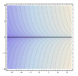
Example 1
Let us find an explicit solution for the PDE $$ Xf(x,y)=g(x,y),\;f(0,y)=0. $$ The flow of $X=\partial_x-y\partial_y$ is given by the solutions of $$ \begin{cases} \dot x = 1\\ \dot y = -y \end{cases}, $$ namely $$ \begin{cases} x(t) = t + x_0\\ y(t) = y_0e^{-t}\\ \end{cases}, $$ where $(x_0,y_0)=(x(0),y(0))$. Hence, the point $(x,y)$ is equal to $\Phi^t_X(0,y_0)$ for $t=x$ and $y_0=ye^{x}$.Example 1
The solution therefore writes as $$ u(x,y) = \int\limits_0^{x}v(t,ye^{x-t})dt $$ E.g. consider the case $v(x,y)=x$. Then $$ u(x,y) = \int\limits_0^{x}tdt = t^2/2\big|^x_0 = x^2/2. $$ Indeed, $u_x-yu_y = x-0=x$. Consider now the case $v(x,y)=y$. Then $$ u(x,y) = \int\limits_0^{x}ye^{x-t}dt = -ye^{x-t}\big|^x_0 = y(e^x-1). $$ Indeed, $u_x-yu_y = ye^x - y(e^x-1) = y$.Example 2
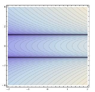
The PDE $$ 2y\,\partial_x f(x,y)+(1-y^2)\,\partial_y f(x,y)=g(x,y) $$ has no global $C^k$ solution, $k=0,1,\dots$, for $g=1\in C^\infty(\Bbb R^2)$.Indeed, the general solution is given by $$ f(x,y)=\frac{1}{2}\ln\left|\frac{1+y}{1-y}\right|+F(x+\ln|1-y^2|)\in L^1_{loc}(\Bbb R^2)\,. $$ This lack of regularity corresponds to the fact that $X$ has no global transversal.
Example 3
Let us solve the PDE $$ x\partial_x u(x,y)-y\partial_y u(x,y) = u(x,y),\; u(x,x)=x^2, $$ on the first quadrant (namely $\Omega=\{x>0,y>0\}$). The flow of $X=x\partial_x-y\partial_y$ is given by $$ \begin{cases} x(t) = x_0e^t\\y(t) = y_0e^{-t}\\ \end{cases} $$ so that $(x,y)=\Phi^t_X(x_0,x_0)$ for $x_0=\sqrt{xy}$ and $t=(\ln x-\ln y)/2$.Example 3
We replace the PDE $Xu=u$ with the system (see slide 4) $$ \begin{cases} X\rho = 1\\ X\left(e^\rho u\right) = 0\ \end{cases} $$ There are no boundary conditions for $\rho$ so we can set $\rho(x,x)=0$. Then the solutions write simply as $$ \rho(x,y) = \int\limits_0^{(\ln x-\ln y)/2}\!\!\!\!\!\!1dt = (\ln x-\ln y)/2 $$ and $$ e^{\rho(x,y)} u(x,y) = \int\limits_0^{(\ln x-\ln y)/2}\!\!\!\!\!\!0dt + x_0^2 = xy. $$ Hence the solution is $$ u(x,y) = y\sqrt{xy}. $$Some basic open problem
- Study the solvability of the cohomological equation on $\Bbb R^3$.
- Study the solvability of the cohomological equation on $\Bbb R^2$ minus some points (namely allow some zero to $X$), e.g. start with one point (namely study the CE on the cilinder).
- Study the solvability of the cohomological equation on compact surfaces.
QuasiLinear PDEs of 1st order
Definition
How to deal with it
There is no general way to solve this equation but we can transform it into a linear equation on some subset of $J^0(\Bbb R^n,\Bbb R)\simeq\Bbb R^{n+1}$, the space of source points and target values, in the following way: given a $\Gamma\subset\Bbb R^n$, the PDE $$X(x,u(x))u(x)=v(x,u(x))\,,\;\;u|_\Gamma=g$$ is equivalent to $$ \begin{cases} \hat X(\hat x)\hat u(\hat x) = 0\\ \hat u(\hat x) = 0\\ \end{cases},\;\;\hat u|_{\hat\Gamma}=\hat g $$ where $$ \begin{array}{rl} \hat x = & \!\!\!\! (x,x^{n+1})\\ \hat u(\hat x)= & \!\!\!\! x^{n+1}-u(x)\\ \hat X(\hat x) = & \!\!\!\! X(x,x^{n+1})+v(x,x^{n+1})\partial_{x^{n+1}}\\ \hat\Gamma = & \!\!\!\! \Gamma\times\Bbb R \subset J^0(\Bbb R^n,\Bbb R)\\ \hat g(\gamma,x^{n+1}) = & \!\!\!\! x^{n+1} - g(\gamma),\;\gamma\in\Gamma.\\ \end{array} $$- $\hat X(x,x^{n+1}) = X(x,x^{n+1})+v(x,x^{n+1})\partial_{x^{n+1}}$ is tangent to $\Lambda_0$ at every point of $\Lambda_0$;
- $\Lambda_0$ can be written as the graph of a function of the first $n$ variables.
Hence, there is always a solution of the original quasilinear PDE close enough to $\Gamma$. Far from $\Gamma$, it is possible that $\Lambda_0$ folds and so we can have more than one point of $\Lambda_0$ that projects on the same point of $\Bbb R^n$, namely we have several possible values for the solution at some point.
Example 1
Let us solve the quasilinear 1st order PDE $$ (y+u(x,y))\partial_x u(x,y) + y\partial_y u(x,y) = x-y,\;\;u(x,1)=1+x. $$ Following the considerations above, we consider the vector field on $\Bbb R^3$ $$\hat X(x,y,z)=(y+z)\partial_x + y\partial_y + (x-y)\partial_z,$$ and look for solutions of $$ \begin{cases} \hat X\hat u(x,y,z) = 0\\ z=u(x,y)\\ \end{cases}, $$ with boundary conditions $$ \hat u(x,1,z)=z-x-1. $$Example 1
The flow of $\hat X$ is given by the solutions of $$ \begin{cases} \dot x = y+z\\ \dot y = y\\ \dot z = x-y\\ \end{cases} $$ Notice that $\dot z+\dot y= x$, so that the solutions of the system above are given by $$ \begin{cases} y(t) = y_0e^t\\ x(t) = x_0\cosh t+(z_0+y_0)\sinh t\\ z(t) + y(t) = x_0\sinh t+(z_0+y_0)\cosh t\\ \end{cases} $$Example 1
Hence, the solutions to $(x,y,z)=\Phi^t_{\hat X}(x_0,1,z_0)$ are given by $$ \begin{cases} t&\!\!\!\!=\ln |y|\\ x_0 &\!\!\!\!= \phantom{-}x\cosh t - (z+y)\sinh t\\ z_0 &\!\!\!\!= -x\sinh t + (z+y)\cosh t-1 \end{cases} $$ so that $$ \hat u(x,y,z) = z_0 - x_0 - 1 = $$ $$ = (z+y-x)\frac{y^2+1}{2y} + (z+y-x)\frac{y^2-1}{2y} - 2 = $$ $$ = (z+y-x)y - 2. $$ Hence the level set $\hat u=0$ is the graph $z = x-y+\frac{2}{y}$,namely our final solution is $$ \hspace{1cm}u(x,y) = x-y+\frac{2}{y}. $$
Remark
Notice that the solution $$ u(x,y)=x-y+2/y $$ is not singular at any point because no trajectory of $\hat X$ that passes through $\hat\Gamma = \{y=1\}$ has intersections with the plane $\{y=0\}$. In other words, the domain of the solution is not the whole $\Bbb R^2$. A direct check shows that the solution is defined only over $\Bbb R\times(0,+\infty)$.Example 2
Let us solve the quasilinear 1st order PDE $$ \partial_x u(x,y) + \partial_y u(x,y) = u^2(x,y),\;\;u(x,0)=g(x). $$ in $\Omega=\Bbb R\times(0,\infty)$. We consider the vector field on $\Bbb R^3$ $$\hat X(x,y,z)=\partial_x + \partial_y + z^2\partial_z,$$ and look for solutions of $$ \begin{cases} \hat X\hat u(x,y,z) = 0\\ z=u(x,y)\\ \end{cases}, $$ with boundary conditions $$ \hat u(x,0,z)=z-g(x). $$Example 2
The flow of $\hat X$ is given by the solutions of $$ \begin{cases} \dot x = 1\\ \dot y = 1\\ \dot z = z^2\\ \end{cases}, $$ namely $$ \begin{cases} x(t) = x_0+t\\ y(t) = y_0+t\\ z(t) = \frac{z_0}{1-z_0t}\\ \end{cases}. $$Example 2
The solution to $(x,y,z)=\Phi^t_{\hat X}(x_0,0,z_0)$ here is given by $$ \begin{cases} t&\!\!\!\!=y\\ x_0 &\!\!\!\!= x-y\\ z_0 &\!\!\!\!= \frac{z}{yz+1} \end{cases}, $$ so that $$ \hat u(x,y,z) = z_0 - g(x_0) = \frac{z}{yz+1} - g(x-y). $$ Hence the level set $\hat u=0$ is the graph $z = \frac{g(x-y)}{1-yg(x-y)}$,namely our final solution is
$$ u(x,y) = \frac{g(x-y)}{1-yg(x-y)}. $$
Remark
In this case, although $X$ is a well defined complete vector field on $\Bbb R^2$, the solution can blow up on some curve on the plane. For instance, if $g(x)=1$, the solution $$ u(x,y)=\frac{1}{1-y} $$ blows up at the line $y=1$. The reason for this behavior is that it is $\hat X$ that is not complete and, in this case, it blows up at $t=1$, when $y=1$. Hence, in this case the solution is defined only in the strip $\Bbb R\times(-\infty,1)$.Remark
As a second example, assume now that $g(x)=x$. The solution $$ u(x,y)=\frac{x-y}{1-y(x-y)} $$ blows up on the line $y(x-y)=1$. In this case, $z(t)$ blows up at $t=1/x_0$, when $y=1/x_0$ and $x=x_0+1/x_0$. Hence, the solution is well defined only in the region $\{y(x-y)<1\}$: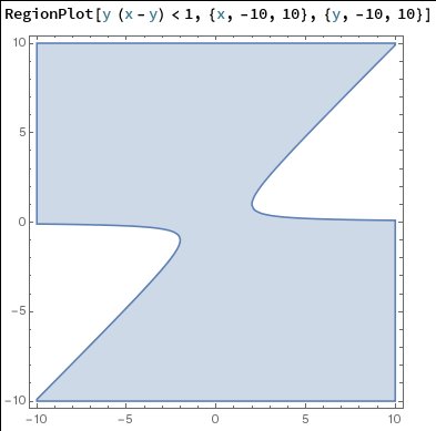
What does this mean?
Just as in case of linear 1st order PDEs, the fact that the solution is defined only in a subset of the plane tells us that the initial conditions given by the problem are not enough to make the solution unique. Outside of the region on which the solution is defined, there are in principle infinitely many functions that satisfy the equation. In order to identify a single one of those, new initial conditions must be specified on some other hypersurface. In principle, it might be needed to specify infinitely many initial conditions to define a unique solution on some open dense set of the plane (the solution might blow up on some hypersurface, as in the cases above).What does this teach us?
Unlike the case of linear 1st order PDEs, with quasilinear 1st order PDEs $$X(x,u(x))u(x)=v(x,u(x))\,,\;\;u|_\Gamma=g$$ in $\Bbb R^n$ the solution might not be defined at every point even when $X(x,u(x))$ does not depend on $u$ and its flow covers the whole plane. In any case, indeed, the domain of the solution is determined by the vec. field $$\hat X(x,x^{n+1})=X(x,x^{n+1})+v(x,x^{n+1})\partial_{x^{n+1}}$$ in $J^0(\Bbb R^n,\Bbb R)\simeq\Bbb R^{n+1}$.Application:
Linear and nonlinear
first order wave equations
The 1st order wave equation
We call wave equation the quasilinear PDE $$ \partial_t u+(u+c)\partial_x u=0,\;\;u(0,x)=f(x) $$ where $c$ is some positive constant.Linear waves
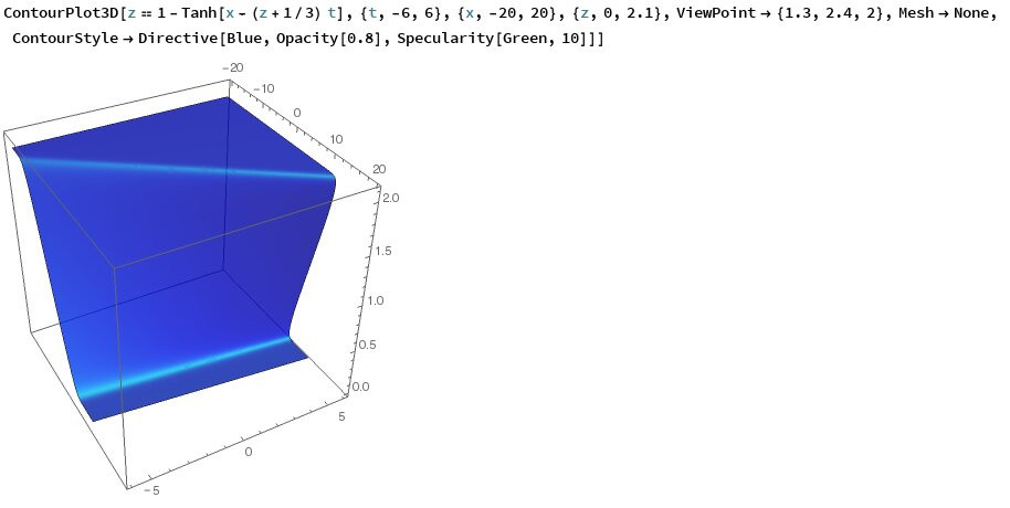
If $u\ll c$ we can approximate this equation by the linear one $$ \partial_t u+c\partial_x u=0,\;\;u(0,x)=f(x)\,, $$ which is called transport equation. In this case $X=\partial_t +c\partial_x$ and its flow is given by $x(t)=ct+x_0$. Hence $(t,x)=\Phi^s_X(0,x_0)$ is solved by $s=t$, $x_0=x-ct$ and so the solution writes $$ u(t,x) = f(x-ct), $$ namely the graph of the solution at any given $t$ is a translation of its graph at any other $t$! The graph moves in the positive $x$ direction as $t$ increases.Linear waves
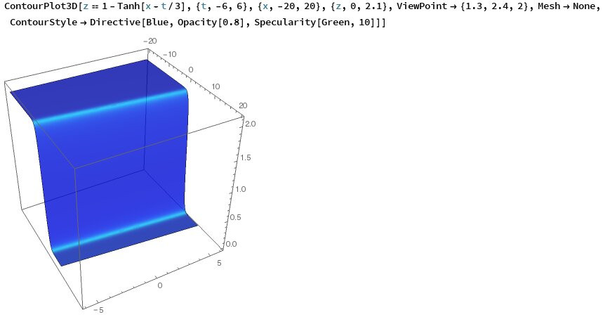
Below we show the set $$\Lambda_0=\{\hat u=0\}=\{y=f(x-ct)\}$$ for $f(x)=\tanh(x)+1$ and $c=1/3$.Since this is a linear equation, $\Lambda_0$ is everywhere the graph of a function:
Nonlinear waves
Now we solve the full equation $$ \partial_t u+(u+c)\partial_x u=0,\;\;u(0,x)=f(x)\,. $$ In this case we consider the vector field $\hat X=\partial_t + (y+c)\partial_x$. Its flow is given by $$ \begin{cases} t(s) &= s + t_0\\ x(s) &= (y_0 + c)s + x_0\\ y(t) &= y_0\\ \end{cases} $$Nonlinear waves
Hence $(t,x,y)=\Phi^s_{\hat X}(0,x_0,y_0)$ is solved by $s=t$, $x_0=x-(y+c)t$, $y_0=y$ and so the solution $\hat u$ writes $$ \hat u(t,x,y) = y_0 - f(x_0) = y - f(x-(y+c)t). $$ The solution $u(t,x)$ then would be the function one gets by solving $$ y - f(x-(y+c)t) = 0 $$ with respect to $y$.Wave breaking
There is nothing, though, stopping the number of solutions of $$ y - f(x-(y+c)t) = 0 $$ from getting larger than 1. In this case therefore there is no uniqueness of the solution anymore since to every solution of the equation above it corresponds a different solution branch.|
The animation on the right shows the set $y - f(x-(y+c)t) = 0$, with $f(x)=4/(4+x^2)$ and $c=2$, in the interval $t\in[0,2.5]$. At about $t=1$ the graph leans so much on its right (like a wave about to break) that the vertical line test starts failing. From the moment on the solution of the PDE is not unique anymore. |
 |
Wave Breaking
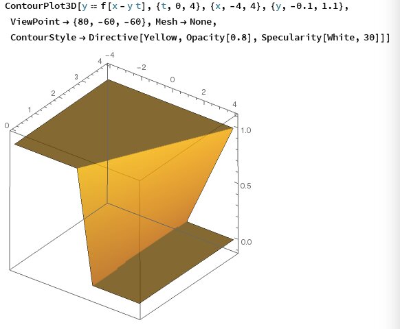
Below we show the set $$\Lambda_0=\{\hat u=0\}=\{y=f(x-(y+c)t)\}$$ for $f(x)=\tanh(x)+1$ and $c=-1/3$.In this case, the top of the wave is faster than its bottom, so after some time the hypersurface $\Lambda_0$ is not anymore the graph of a function of $(t,x)$:
What do we learn from here?
Except in the simple case of linear equations, it makes more sense to say that the solution of a quasilinear 1st order PDE on $\Bbb R^n$ is a hypersurface $$ \Lambda_0\subset J^0(\Bbb R^n,\Bbb R) $$ such that $\hat X$ is tangent to $\Lambda_0$ at each of its points.Application:
Conservation Laws in $\Bbb R$
Conservation Laws
Now we study in same detail the case of the 1st order quasilinear PDE on $(0,\infty)\times\Bbb R$: $$ \partial_t f+\partial_x F(f)=0\,,\;\;f(0,x)=g(x) $$ Notice that this becomes the wave equation at $c=0$ when $F(x)=x^2/2$. This specific PDE is called Burgers Equation. The name comes from the fact that, if $f$ is the density of some quantity and $F$ represents the flow rate of that quantity, then the PDE $f_t+(F(f))_x=0$ expresses differentially the fact that $$ \frac{d\phantom{t}}{dt}\int\limits_{x_1}^{x_2}f(t,\xi)d\xi=\int\limits_{x_1}^{x_2}f_t(t,\xi)d\xi = - \int\limits_{x_1}^{x_2}\partial_\xi\left(F(f(t,\xi))\right)d\xi = F(f(t,x))\bigg|^{x_1}_{x_2} $$ namely the "charge" $Q=\int_{x_1}^{x_2}f(t,\xi)d\xi$ in the interval $[x_1,x_2]$ changes by the difference of the flow of $f$ at its boundary. In particular, if the flow of $f$ at the boundary is the same, $Q$ is constant.Weak solutions
As we pointed out in case of the wave equation, often quasilinear equations have regular (at least continuous) solutions only in a small neighborhood of the initial hypersurface $\Gamma$, that here is always the $t=0$ hyperplane. Yet, many systems of physical importance can be modeled by conservation laws and the discontinuities of their solutions have a physical meaning.It is important therefore to give a meaning to "discontinuous solutions of a differential equation". Discontinuous solutions of PDEs are called weak solutions. In order to define them we must re-write the PDE into integral form.
Integral Form
Let $v$ be any smooth function with compact support in $[0,\infty)\times\Bbb R$. Then $$ \int_{[0,\infty)\times\Bbb R}\left[f_t+[F(f)]_x\right]v\,dtdx=0 $$ and, integrating by parts and using the fact that $v=0$ at the boundary, $$ \int_{[0,\infty)\times\Bbb R}\left[f\,v_t+F(f)\,v_x\right]\,dtdx + \int_{[0,\infty)}g(x)v(0,x)\,dx=0. $$ A function $f\in L^\infty([0,\infty)\times\Bbb R)$ satisfying the integral equation above is a weak solution of the PDE.Behavior of a weak solution at a discontinuity
Given a weak solution $f$ which is discontinuous over a hypersurface $\gamma$, is there a compatibility condition for the values of $f$ on opposite sides of $\gamma$? The answer is positive and these conditions are called Rankine-Hugoniot conditions: Theorem If $f$ is a weak solution that is discontinuous across $\gamma$ and smooth everywhere else, then $$ \frac{F(f_+)-F(f_-)}{f_+-f_-}=\gamma'(t), $$ where $f_+$ is the limit of $f$ when $(t,x)$ approaches $\gamma(t)$ from one side (which we call positive) and $f_-$ is the limit of $f$ when $(t,x)$ approaches $\gamma(t)$ from the opposite side (which we call negative).Example 1
$$\partial_t f+ f\partial_x f=0\,,\;\;f(0,x) = \begin{cases}0,& x>1\\1-x,&0\leq x\leq1\\1,& x<0\end{cases}$$ Here $F(x)=x^2/2$ and $$ \hat X(t,x,y) = \partial_t + y\partial_x $$ whose flow is the solution of $$ \begin{cases} \dot t = 1\\ \dot x = y\\ \dot y = 0\\ \end{cases} $$ namely $$ \begin{cases} t = \lambda\\ x = y_0\lambda+x_0\\ y = y_0\\ \end{cases} $$Example 1
Hence the projection of the characteristics on the $(t,x)$ plane are: $$ x(t)= \begin{cases} x_0,& x_0 > 1\\ (1-x_0)t+x_0,&0\leq x_0\leq1\\ t+x_0,& x_0<0\end{cases}$$ No collision can arise between characteristics starting at $x_0<0$ and $0\leq x_0\leq 1$ but both of them intersect every characteristic starting at $x_0>1$. The first collision takes place at $t=1$ -- indeed, all lines starting at $0\leq x_0\leq1$ pass through $(1,1)$. For $t\leq 1$, the (smooth!) solution is $$ f(t,x) = \begin{cases} 0,& x > 1\\ \frac{1-x}{1-t},&t\leq x\leq1\\ 1,& x < t\\ \end{cases} $$Example 1
Example 1
The discontinuity of $f$ must be on some half-line $\ell(t)$ through the point $(1,1)$ and the value of $f$ on the opposite sides of $\ell(t)$ must be 0 and 1. By the Rankine-Hugoniot conditions, we must have that $$ \ell'(t) = \frac{F(f_+)-F(f_-)}{f_+-f_-} = \frac{1/2-0/2}{1-0} = \frac{1}{2} $$ Hence, the discointinuity line is $\ell(t) = (1+t)/2$. In other words, the Rankine-Hugoniot conditions determine univoquely the line of discontinuity and therefore the unique weak solution to the problem.Example 2
$$\partial_t f+ f\partial_x f=0\,,\;\;f(0,x) = \begin{cases}1,& x>1\\0,& x<0\end{cases}$$ This is again Burgers' PDE with different initial conditions. In this case, the projection of the characteristics on the $(t,x)$ plane are: $$ x(t)= \begin{cases} t+x_0,& x_0 > 0\\ x_0,& x_0<0\end{cases}$$ Hence, there are no collisions among trajectories and there is a regular solution in the region covered by the characteristics: $$ f(t,x) = \begin{cases} 1,& x > t\\ 0,& x < 0\\ \end{cases} $$ No value for $f$ follows from the equation in the region $\{0 < x < t\}$.So, where is the problem?
The problem is: is there any way to extend uniquely the regular solution to a weak solution defined over the whole plane? The answer is positive under extra ("entropy") conditions that we will give in the next slide. Under those conditions, the unique solution of this PDE is given by the "rarefaction wave" $$ f(t,x) = \begin{cases} 1,& x > t\\ x/t,& 0\leq x \leq t\\ 0,& x < 0\\ \end{cases} $$Uniqueness of Weak solutions
Theorem Assume that $F\in C^\infty(\Bbb R)$ is convex, e.g. $\inf F''(x) >0$.Then the PDE $$f_t+(F(f))_x=0\,,\;\;f(0,x)=g(x)\in L^\infty(\Bbb R)$$ has at most one weak solution satisfying the "entropy condition" $$ f(t,x+h)-f(t,x)\leq C\left(1+\displaystyle\frac{1}{t}\right)h $$ for some $C\geq0$ and almost all $x\in\Bbb R$ and $t,h\in(0,\infty)$.
Example (Riemann Problem)
The unique weak solution of $$f_t+(F(f))_x=0\,,\;\;f(0,x)=\begin{cases}f_-,&x<0\\ f_+,&x>0\\ \end{cases}\,,$$ where $f_-\neq f_+$ are two constants, is: if $f_->f_+$, $$ f(t,x)=\begin{cases} f_-,&x<\sigma t\\ f_+,&x>\sigma t\\ \end{cases},\;\;\hbox{where}\;\;\sigma=\frac{F(f_+)-F(f_-)}{f_+-f_-}\;; $$ if $f_- < f_+$, $$ f(t,x)= \begin{cases} f_-,&x < F'(f_-) t\\ G\left(\frac{x}{t}\right),&F'(f_-)t < x < F'(f_+)t\\ f_+,&x>F'(f_+) t\\ \end{cases},\;\;\hbox{where}\;\;G=(F')^{-1}\;. $$Fully nonlinear 1st order PDEs
Definition
A natural map $F\to X_F$
The reason why we can actually solve this fully nonlinear kind of equations is that, for any function $F$, there exists a natural vector field $X$ on $J^1(\Bbb R^n,\Bbb R)$ tangent to the level sets of $F$, namely such that $XF=0$. This vector field is: $$ X_F(x^\alpha,z,p_\alpha) = \frac{\partial F}{\partial p_\alpha}\frac{\partial\phantom{x^\alpha}}{\partial x^\alpha} + p_\alpha\frac{\partial F}{\partial p_\alpha}\frac{\partial\phantom{z}}{\partial z}-\left(\frac{\partial F}{\partial x^\alpha}+p_\alpha\frac{\partial F}{\partial z}\right)\frac{\partial\phantom{p_\alpha}}{\partial p_\alpha} $$ Indeed, $$ X_FF = \frac{\partial F}{\partial p_\alpha}\frac{\partial F}{\partial x_\alpha} + p_\alpha\frac{\partial F}{\partial p_\alpha}\frac{\partial F}{\partial z}-\left(\frac{\partial F}{\partial x^\alpha}+p_\alpha\frac{\partial F}{\partial z}\right)\frac{\partial F}{\partial p_\alpha} = 0. $$ We will see below the deep geometric origin of this association $F\to X_F$.How to solve the equation
The set $F_0=\{F(x,z,p)=0\}$ is (for a generic $F$) a regular hypersurface of $J^1(\Bbb R^n,\Bbb R)$ [namely $\dim F_0=2n$]. Consider now the initial condition $u|_{\Gamma_0}=g$. Using $g$ and $F$, we can build a map $\hat g:\Gamma_0\to J^1(\Bbb R^n,\Bbb R)$ such that $\hat\Gamma_0=\hat g(\Gamma_0)\subset F_0$. For instance, assume $\Gamma_0=\{x^n=0\}$ (we can always make it so locally with a coordinate change). Then set $\tilde x=(x^1,\dots,x^{n-1})$ and define $$ \hat g(\tilde x) = (\tilde x,0,g(\tilde x),\partial_{x^1}g(\tilde x),\dots,\partial_{x^{n-1}}g(\tilde x),\xi(\tilde x)), $$ where $\xi(\tilde x)$ is a solution of the implicit equation $$ F(\tilde x,0,g(\tilde x),\partial_{x^1}g(\tilde x),\dots,\partial_{x^{n-1}}g(\tilde x),\xi(\tilde x))=0. $$ Recall that the implicit function thm grants that such a smooth function always exists in some nbhd of a point $f_0\in F_0$ when $\partial_{p_n}F\neq 0$ at $f_0$.How to solve the equation
Finally, assume that $X_F$ is never tangent at $\hat\Gamma_0$ and consider $$ \hat\Gamma = \cup_{t\in\Bbb R}\Phi^t_{X_F}(\hat\Gamma_0)\subset F_0, $$ namely $\hat\Gamma$ is the $n$-dimensional submanifold spanned by $\hat\Gamma_0$ under the flow of $X_F$. Since $\hat\Gamma_0$ projects nicely over $\Gamma_0$ (i.e. there is only one point of $\hat\Gamma_0$ over every point of $\Gamma_0$), then the same will happen to every $\Phi^t_{X_F}(\hat\Gamma_0)$ for $t$ small enough. It can be proved that, at least for small times $t$, $\hat\Gamma$ is the 1-graph of a function $u$, namely $\hat\Gamma=\{(x,u(x),\partial u(x)\}$ for some function $u:\Bbb R^n\to\Bbb R$. This $u$ is a sulution to $F(x,u(x),\partial u(x))=0$ with boundary conditions $u_{\Gamma_0}=g$.Example 1
Let us solve the nonlinear 1st order PDE $$ u_x u_y-u=0\,,\Gamma_0=\{y=-x\}\,,\;u(x,-x)=1. $$ Here the function $F:J^1(\Bbb R^2,\Bbb R)\to\Bbb R$ is given by the polynomial $$ F(x,y,z,p_x,p_y) = p_xp_y-z $$ and the corresponding vector field is $$ X_F = p_y\frac{\partial\phantom{x}}{\partial x} + p_x\frac{\partial\phantom{y}}{\partial y} + 2 p_xp_y\frac{\partial\phantom{z}}{\partial z} + p_x \frac{\partial\phantom{p_x}}{\partial p_x} + p_y \frac{\partial\phantom{p_y}}{\partial p_y} $$Example 1
The flow of $X_F$ is given by the solution of the ODE system $$ \begin{cases} \dot x &= p_y\\ \dot y &= p_x\\ \dot z &= 2p_xp_y\\ \dot p_x &= p_x\\ \dot p_y &= p_y\\ \end{cases} $$ namely $$ \begin{cases} p_x(t)&=p_{x,0}e^t\\ p_y(t)&=p_{y,0}e^t\\ x(t) &= p_{y,0}(e^t-1)+x_0\\ y(t) &= p_{x,0}(e^t-1)+y_0\\ z(t) &= p_{x,0}p_{y,0}(e^{2t}-1)+z_0\\ \end{cases} $$Example 1
Now we look for the function $\hat g:\Bbb R\to F_0\subset J^1(\Bbb R^2,\Bbb R)$, namely a function $$ \hat g(x) = (x,-x,1,a(x),b(x)) $$ such that- $F(x,-x,1,a(x),b(x))=0$
- $a(x)x'+b(x)(-x)'=(u(x,-x))'=0$
- $F_{p_x}(x,-x,1,a(x),b(x))(-x')-F_{p_y}(x,-x,1,a(x),b(x))(x')\neq0$
- $a(x)b(x)=1$
- $a(x)=b(x)$
- $a(x)+b(x)\neq0$.
Example 1
Hence we can take either $$ \hat g(x) = (x,-x,1,1,1) $$ or $$ \hat g(x) = (x,-x,1,-1,-1). $$ Each of these two choices gives us a different version of $\hat\Gamma_0$. From the first we get that $$ \hat\Gamma=\bigcup_{t\in\Bbb R} \Gamma_t=\bigcup_{(t,x_0)\in\Bbb R^2}\Phi^t_{X_F}(x_0,-x_0,1,1,1) $$ is the surface $$ \begin{cases} x(t,x_0) &= e^t-1+x_0\\ y(t,x_0) &= e^t-1-x_0\\ z(t,x_0) &= e^{2t}-1\\ p_x(t,x_0)&=e^t\\ p_y(t,x_0)&=e^t\\ \end{cases} $$Example 1
This surface is the 1-graph of the function $$ z = e^{2t}-1 = \frac{(x+y+2)^2}{4}, $$ namely the function $$ u(x,y) = \frac{(x+y+2)^2}{4} $$ is a solution of $$ u_x u_y-u=0\,,\Gamma_0=\{y=-x\}\,,\;u(x,-x)=1. $$ The second possible choice for $\hat\Gamma$ gives a second solution, namely $$ u(x,y) = \frac{(x+y-2)^2}{4} $$ No other solution is possible for this PDE.Digression:
Lagrangian and Hamiltonian mechanics
Fermat's principle in Optics
Already around the year 1000, Ibn al-Haytham understood that light rays move from a point $A$ to a point $B$ in such a way to minimize the travel time. The statement of this principle in modern form was stated by Fermat in 1662. In modern notation, it says that light trajectories minimize the quantity $$ S = \int\limits_A^B n(x)ds $$ where $n$ is the ratio between the speed of light in vacuum and the speed of light in the medium (e.g. air or glass). For example, if $A$ and $B$ lie in two different media separated by a straigh line, in order to minimize the time the ray has to obey the laws of refraction (read this interesting article!).Least action principle in mechanics
Surprisingly, Newton's law $F=ma$ for conservative forces (for which the kinetic energy $T=mv^2/2$ is conserved) obeys a similar principle. Recall that a force field $F$ is conservative if $F=-\nabla U$ for some smooth function $U:\Bbb R^n\to\Bbb R$, so that Newton's law writes as $$ m\ddot x^\alpha=-\partial_\alpha U. $$ Consider the Lagrangian function $L=T-U$, namely $$ L(x^\alpha,v^\alpha)=\frac{1}{2}g_{\alpha\beta}v^\alpha v^\beta - U(x^\alpha) \,,\; g_{\alpha\beta} = m \delta_{\alpha\beta} $$ Then the solutions of $m\ddot x=F,x(t_0)=x_0,x(t_1)=x_1$ are extremal for $$ S[\gamma] = \int_\gamma L(x,\dot x)dt $$ over all smooth paths $\gamma:[t_0,t_1]\to\Bbb R^n$ s.t. $\gamma(t_0)=x_0$, $\gamma(t_1)=x_1$.Euler-Lagrange equations
Indeed, if you consider a 1-parameter family of such paths $\gamma_\epsilon$ and set $\delta=d/d\epsilon|_{\epsilon=0}$, then $$ \delta S[\gamma_0]=\int_{t_0}^{t_1}\delta L(\gamma_\epsilon(t),\dot\gamma_\epsilon(t))dt= $$ $$ =\int_{t_0}^{t_1}\left(\frac{\partial L}{\partial x^\alpha}\delta\gamma(t)+ \frac{\partial L}{\partial v^\alpha}\delta\dot\gamma(t)\right)dt= $$ $$ =\int_{t_0}^{t_1}\left(\frac{\partial L}{\partial x^\alpha}- \frac{d\phantom{t}}{dt}\frac{\partial L}{\partial v^\alpha}\right)\delta\gamma(t)dt, $$ namely $$ \delta S[\gamma_0]=0\;\;\;\hbox{ iff }\;\;\; \frac{d\phantom{t}}{dt}\frac{\partial L}{\partial v^\alpha}=\frac{\partial L}{\partial x^\alpha}. $$Euler-Lagrange equations
Explicitly, $$ \frac{\partial L}{\partial v^\alpha} = g_{\alpha\beta}v^\beta \,,\; \frac{\partial L}{\partial x^\alpha} = -\partial_\alpha U $$ so that the EL equations $$ \frac{d\phantom{t}}{dt}\frac{\partial L}{\partial v^\alpha}=\frac{\partial L}{\partial x^\alpha}. $$ translate precisely into Newton's law $$ m\delta_{\alpha\beta}\ddot x^\beta = -\partial_\alpha U. $$Lagrangian mechanics
The Lagrangian point of view though is far superior because it generalizes easily to a much wider setting: given any function $$ L:J^1(\Bbb R,\Bbb R^n)\to\Bbb R $$ we associate to it an ODE system given by $$ \frac{d\phantom{t}}{dt}\frac{\partial L}{\partial v^\alpha}=\frac{\partial L}{\partial x^\alpha} $$ whose solutions are all extremal for the functional $$ S[\gamma] = \int_\gamma L(t,x,v)dt = \int_{t_0}^{t_1} L(j^1_t\gamma)dt . $$Hamiltonian mechanics
In physics, though, even more important than the velocity $\dot x$ is the momentum $p=m\dot x$. From a geometrical point of view, this corresponds to passing from the tangent to the cotangent space. Consider indeed the momenta $\displaystyle p_\alpha = \frac{\partial L}{\partial v^\alpha}$. If $L$ is convex with respect to the $v^\alpha$, this defines a bijective correspondance between $\dot x$ and $p$.Example: when $L=T-U$ and $T=g_{\alpha\beta}v^\alpha v^\beta/2$, then $p_\alpha=g_{\alpha\beta}v^\beta$. Now define the Hamiltonian function $$ H(x^\alpha,p_\alpha) = p_\alpha v^\alpha - L(x^\alpha,v^\alpha), $$ where on the r.h.s. $v^\alpha$ is intended as function of $p_\alpha$.
Hamiltonian mechanics
Now, by definition $$ dH = \frac{\partial H}{\partial x^\alpha}dx^\alpha + \frac{\partial H}{\partial p_\alpha}dp_\alpha $$ but, since $H(x,p)=p_\alpha v^\alpha-L(x,v)$ and $p_\alpha =\frac{\partial L}{\partial v^\alpha}$, we also have that $$ dH = p_\alpha d\dot x^\alpha + \dot x^\alpha dp_\alpha - \frac{\partial L}{\partial x^\alpha}dx^\alpha - \frac{\partial L}{\partial v^\alpha}d\dot x^\alpha = $$ $$ = \dot x^\alpha dp_\alpha - \frac{d\phantom{t}}{dt} \frac{\partial L}{\partial v^\alpha}dx^\alpha = \dot x^\alpha dp_\alpha - \dot p_\alpha dx^\alpha $$ Hence on $T^*\Bbb R^n$ the EL equations become the Hamiltonian equations $$ \begin{cases} \dot x^\alpha &=\displaystyle \phantom{-}\frac{\partial H}{\partial p_\alpha}\\ \dot p_\alpha &=\displaystyle -\frac{\partial H}{\partial x^\alpha}\\ \end{cases} $$Conservation of Energy
The Hamiltonian is the energy function for the system defined by the corresponding Lagrangian and it is preseved on the solutions of the equations of motion. Indeed the corresponding vector field is $$ X_H = \frac{\partial H}{\partial p_\alpha}\frac{\partial\phantom{H}}{\partial x^\alpha} - \frac{\partial H}{\partial x^\alpha}\frac{\partial\phantom{H}}{\partial p_\alpha} $$ and so $$ X_H(H) = \frac{\partial H}{\partial p_\alpha}\frac{\partial H}{\partial x^\alpha} - \frac{\partial H}{\partial x^\alpha}\frac{\partial H}{\partial p_\alpha} = 0. $$The case $\partial_z F=0$,
a.k.a.
the Hamilton-Jacobi equation
Wave fronts
Consider a point-like source at $x_0$. The wave-front $\Phi^t(x_0)$ is the set of all points reached by the light after a time $t$. There is a strong relation between the rays and wave-fronts points of view (Huygen's principle): if rays move according to Fermat's principle, for all $t'>t$ the wave-front $\Phi^{t'}(x_0)$ is the envelope of all wave fronts emanating from all points of $\Phi^{t}(x_0)$.
Wave fronts in mechanics
The dualism ray/wave front arises also in mechanics and it corresponds exactly to the method of integration of first order PDEs: rays correspond to the integral trajectories of the vector field $X_F$ while the wave fronts correspond to the surfaces $\hat\Gamma_t=\Phi^t_{X_F}(\hat\Gamma_0)$. In concrete, consider "at time 0", a function $S_0:\Bbb R^n\to\Bbb R$ and set $$ \hat\Gamma_0 = \{(x^\alpha,\partial_\alpha S(x))\,|\;x\in\Bbb R^n\}\subset T^*\Bbb R^n. $$ Remark: $\hat\Gamma_0$ is a $n$-dimensional surface inside a $2n$-dimensional space. Given a Hamiltonian $H:T^*\Bbb R^n\to\Bbb R$, the Hamiltonian flow $\Phi^t_{X_H}$ will move points of $\hat\Gamma_0$ around so that $\hat\Gamma_t=\Phi^t_{X_H}(\hat\Gamma_0)$ is the "wave-front" at time $t$. The union of all wave-fronts is a $n+1$ dimensional surface $$ \hat\Gamma = \{\left(t,\Phi^t_{X_H}(x_0,p_0)\right)\,|\;(x_0,p_0)\in\hat\Gamma_0,\,t\in\Bbb R\}\subset\Bbb R\times T^*\Bbb R^n. $$Wave fronts in mechanics
Now consider the action function, namely the function $$ S_{\hat\Gamma_0}(t,x) = \int_{\bar\gamma}p_\alpha dx^\alpha - H(x^\alpha,p_\alpha)dt $$ where $\bar\gamma$ is the solution of the Hamilton equations that passes through $x$ at time $t$ and intersects $\hat\Gamma_0$ at time $0$. Remark: this solution is unique if $t$ is "small enough". The following intuitive relation can be proved rigorously: $$ dS_{\hat\Gamma_0} = p_\alpha(x) dx^\alpha - H(x^\alpha,p_\alpha(x))dt. $$The Hamilton-Jacobi equation
Remark: $S$ is a function of $(t,x^\alpha)$ only! Here by $p_\alpha$ we mean the equations $p_\alpha=p_\alpha(x)$ of the graph of the surface $\hat\Gamma_t=\Phi^t_{X_H}\hat\Gamma_0$ (they are well-defined for $t$ small enough). Since $dS_{\hat\Gamma_0} = p_\alpha dx^\alpha - Hdt$, the function $S_{\hat\Gamma_0}$ satisfies $$ \frac{\partial S}{\partial t} + H\left(x^\alpha,\frac{\partial S}{\partial x^\alpha}\right) = 0. $$ This 1st order PDE is called the Hamilton-Jacobi equation.The corresponding characteristic vector field is $$ X = \frac{\partial\phantom{p}}{\partial t} + p_\alpha\frac{\partial H}{\partial p_\alpha}\frac{\partial\phantom{p}}{\partial z} + \frac{\partial H}{\partial p_\alpha}\frac{\partial\phantom{p}}{\partial x^\alpha} - \frac{\partial H}{\partial x^\alpha}\frac{\partial\phantom{p}}{\partial p_\alpha}, $$ so that the "interesting part" of its flow is the Hamiltonian flow.