Trigonometric functions are used to model many phenomena, including sound waves, vibrations of strings, alternating electrical current, and the motion of pendulums. In fact, almost any repetitive, or cyclical, motion can be modeled by some combination of trigonometric functions. In this section, we define the six basic trigonometric functions and look at some of the main identities involving these functions.
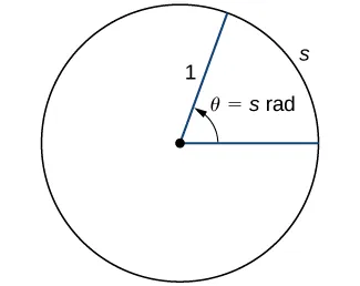
To use trigonometric functions, we first must understand how to measure the angles. Although we can use both radians and degrees, radians are a more natural measurement because they are related directly to the unit circle, a circle with radius 1. The radian measure of an angle is defined as follows. Given an angle 𝜃, let 𝑠 be the length of the corresponding arc on the unit circle (Figure 1.30). We say the angle corresponding to the arc of length 1 has radian measure 1.
Since an angle of 360° corresponds to the circumference of a circle, or an arc of length \(2\pi\text{,}\) we conclude that an angle with a degree measure of 360° has a radian measure of \(2\pi\text{.}\) Similarly, we see that 180° is equivalent to \(\pi\) radians. Table 1.3.2 shows the relationship between common degree and radian values.
Table1.3.2.Common Angles Expressed in Degrees and Radians.
Trigonometric functions allow us to use angle measures, in radians or degrees, to find the coordinates of a point on any circle—not only on a unit circle—or to find an angle given a point on a circle. They also define the relationship among the sides and angles of a triangle.
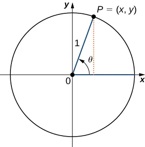
To define the trigonometric functions, first consider the unit circle centered at the origin and a point 𝑃=(𝑥,𝑦) on the unit circle. Let 𝜃 be an angle with an initial side that lies along the positive 𝑥-axis and with a terminal side that is the line segment 𝑂𝑃. An angle in this position is said to be in standard position (Figure 1.31). We can then define the values of the six trigonometric functions for 𝜃 in terms of the coordinates 𝑥 and 𝑦.
Let 𝑃=(𝑥,𝑦) be a point on the unit circle centered at the origin 𝑂. Let 𝜃 be an angle with an initial side along the positive 𝑥-axis and a terminal side given by the line segment 𝑂𝑃. The trigonometric functions are then defined as
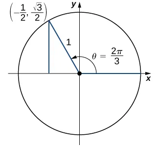
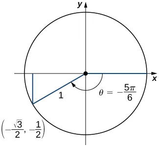
Table 1.3.6 shows the values of sine and cosine at the major angles in the first quadrant. From this table, we can determine the values of sine and cosine at the corresponding angles in the other quadrants. The values of the other trigonometric functions are calculated easily from the values of sin𝜃 and cos𝜃.
Table1.3.6.Values of sin𝜃 and cos𝜃 at Major Angles 𝜃 in the First Quadrant.
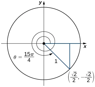
An angle \(𝜃=15𝜋/4=2𝜋+7𝜋/4\text{.}\) Therefore, this angle corresponds to more than one revolution, as shown. Knowing the fact that an angle of \(7𝜋/4\) corresponds to the point (√2/2,−√2/2), we can conclude that
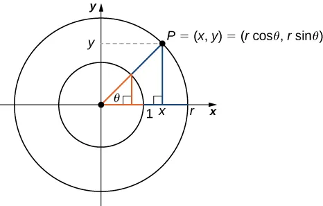
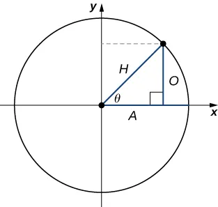
As mentioned earlier, the ratios of the side lengths of a right triangle can be expressed in terms of the trigonometric functions evaluated at either of the acute angles of the triangle. Let 𝜃 be one of the acute angles. Let 𝐴 be the length of the adjacent leg, 𝑂 be the length of the opposite leg, and 𝐻 be the length of the hypotenuse. By inscribing the triangle into a circle of radius 𝐻, as shown in Figure 1.33, we see that 𝐴,𝐻, and 𝑂 satisfy the following relationships with 𝜃:
Figure1.3.11.By inscribing a right triangle in a circle, we can express the ratios of the side lengths in terms of the trigonometric functions evaluated at 𝜃.
A wooden ramp is to be built with one end on the ground and the other end at the top of a short staircase. If the top of the staircase is 4 ft from the ground and the angle between the ground and the ramp is to be 10°, how long does the ramp need to be?
A trigonometric identity is an equation involving trigonometric functions that is true for all angles 𝜃 for which the functions are defined. We can use the identities to help us solve or simplify equations. The main trigonometric identities are listed next.
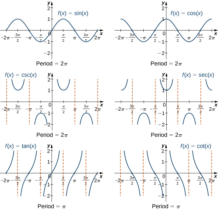
We have seen that as we travel around the unit circle, the values of the trigonometric functions repeat. We can see this pattern in the graphs of the functions. Let 𝑃=(𝑥,𝑦) be a point on the unit circle and let 𝜃 be the corresponding angle . Since the angle \(𝜃\) and \(𝜃+2\pi\) correspond to the same point 𝑃, the values of the trigonometric functions at \(𝜃\) and at \(𝜃+2\pi\) are the same. Consequently, the trigonometric functions are periodic functions. The period of a function 𝑓 is defined to be the smallest positive value 𝑝 such that 𝑓(𝑥+𝑝)=𝑓(𝑥) for all values 𝑥 in the domain of 𝑓. The sine, cosine, secant, and cosecant functions have a period of \(2\pi\text{.}\) Since the tangent and cotangent functions repeat on an interval of length \(\pi\text{,}\) their period is \(\pi\) (Figure 1.3.13).
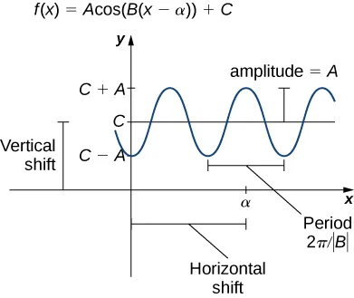
In Figure 1.3.15, the constant 𝛼 causes a horizontal or phase shift. The factor 𝐵 changes the period. This transformed sine function will have a period 2\pi/|𝐵|. The factor 𝐴 results in a vertical stretch by a factor of |𝐴|. We say |𝐴| is the “amplitude of 𝑓.” The constant 𝐶 causes a vertical shift.
Notice in Figure 1.3.9 that the graph of \(𝑦=\cos𝑥\) is the graph of \(𝑦=\sin𝑥\) shifted to the left \(\pi/2\) units. Therefore, we can write \(\cos𝑥=\sin(𝑥+\pi/2)\text{.}\) Similarly, we can view the graph of \(𝑦=\sin𝑥\) as the graph of \(𝑦=\cos𝑥\) shifted right \(\pi/2\) units, and state that \(\sin𝑥=\cos(𝑥−\pi/2)\text{.}\)
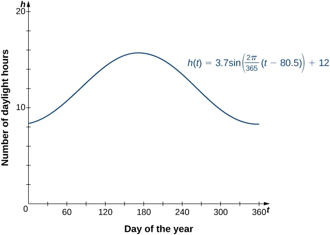
A shifted sine curve arises naturally when graphing the number of hours of daylight in a given location as a function of the day of the year. For example, suppose a city reports that June 21 is the longest day of the year with 15.7 hours and December 21 is the shortest day of the year with 8.3 hours. It can be shown that the function