Section 2.6 Finite Elements Method
The Finite Differences method has a big problem: it is very natural to study PDEs defined over a Cartesian product but it is very unnatural to apply to any other shape, for instance even just a triangle or a disc, let alone more complicated ones. The Finite Elements method was devised exactly to overcome this problem: it is a method that applies in the same way to any kind of shape. The method is based on the following observations from Functional Analysis:- The usual spaces of functions to whom PDEs solutions belong, namely the spaces of \(C^k\) functions, are all (infinite-dimensional!) vector spaces and in each such spaces one can define some kind of scalar product.
- A complete vector space \(H\) endowed with a scalar product \(\langle,\rangle\) is called Hilbert space. Each separable Hilbert space, namely a Hilbert space with a countable dense set, has a countable basis\begin{equation*} \{e_1,\dots,e_n,\dots\}\text{,} \end{equation*}so that every \(v\in H\) can be written uniquely as\begin{equation*} v=\sum_{i=1}^\infty v_i e_i, \end{equation*}where\begin{equation*} v_i=\langle v, e_i\rangle. \end{equation*}This always happens when considering spaces of smooth functions on compact (namely closed and bounded) sets \(\Omega\subset\bR^n\text{.}\) Notice that this is not a restriction for us since numerically we can only investigate PDEs defined on bounded sets.
- All differential operators are linear operators between functional spaces, for instance\begin{equation*} \frac{\partial\phantom{x}}{\partial x}:C^k(\Omega)\to C^{k-1}(\Omega) \end{equation*}and, more importantly,\begin{equation*} \frac{\partial\phantom{x}}{\partial x}:C^\infty(\Omega)\to C^{\infty}(\Omega) \end{equation*}
- Complete \(C^\infty(\Omega)\) with respect to the distance induced by a given scalar product. Denote by \(H\) the complete space.
- Choose a basis \(\{e_1,\dots,e_n,\dots\}\) for \(H\text{.}\) With respect to this basis, the PDE becomes an infinite linear system.
- Truncate the basis to a finite number of elements. Now the linear system is finite and can be solved numerically. The larger the number of basis elements kept, the more accurate the approximation will be.
Subsection 2.6.1 Example 1 - ODEs
Consider the space
\begin{equation*}
V=C^\infty[0,1]
\end{equation*}
of all functions
\begin{equation*}
u:[0,1]\to\Bbb R
\end{equation*}
that are continuous on the whole interval \(D=[0,1]\) together with their derivatives of any order. \(V\) is a vector space since, if \(u,v\in V\text{,}\) then also any linear combination \(\alpha u+\beta v\in V\) for every \(\alpha,\beta\in\Bbb R\text{.}\) The dimension of this space, though is infinite! For example
\begin{equation*}
s_n(x) = \sin(2\pi n x)\,,\;c_n(x)=\cos(2\pi n x)\,,\; n=1,2,3,\dots
\end{equation*}
is a set of infinitely many linearly independent elements of \(V\text{.}\) In fact, every function in \(V\) can be developed in Fourier series:
\begin{equation*}
u=\sum_{n=1}^\infty \left(u_{s,n} s_n+u_{c,n} c_n\right),
\end{equation*}
where the convergence is uniform. Notice, though, that this space is not a Hilbert space because there is no scalar product that makes it complete. Since we do want nevertheless a scalar product, we introduce here the following one:
\begin{equation*}
\langle f,g \rangle = \displaystyle\int_0^1\!\!\!f(x)g(x)dx\,.
\end{equation*}
The space \(V\) with the scalar product \(\langle,\rangle\) is a pre-Hilbert space, namely \(V\) is like an Euclidean space but it is not complete (just like \(\Bbb Q^n\) is not complete with respect to the Euclidean distance) because Cauchy sequences \(\{u_n\}\) of \(V\) might not converge to elements of \(V\) The completion of \(V\) with respect to \(\langle,\rangle\) is called \(L^2[0,1]\) and is the space of all measurable functions \(u\) such that
\begin{equation*}
\|u\|^2=\int_0^1|u(x)|^2 dx<\infty\,.
\end{equation*}
Consider now the following equation in \(V\text{:}\)
\begin{equation*}
-u''(x)+r(x)u(x)=f(x)\,,\;x\in[0,1]\,,\;\;u(0)=u(1)=0\,,
\end{equation*}
where \(f,r\in V\text{.}\) This is a linear equation in \(V\) and can be written as
\begin{equation*}
Au=f\,,\;u\in C^\infty_0[0,1]
\end{equation*}
where \(A\) is the linear operator from \(V\) to itself
\begin{equation*}
-\frac{d^2}{dx^2}+r(x)
\end{equation*}
and \(C^\infty_0[0,1]\) is the subset of smooth functions that are zero at \(x=0,1\text{.}\) We need a few steps to get to the weak form of this linear equation. First we take the scalar product with a \(s\in C^\infty_0[0,1]\text{,}\) so we get
\begin{equation*}
-\langle u'',s\rangle + \langle r\cdot u, s\rangle = \langle f,s\rangle\,.
\end{equation*}
Then we integrate by parts the first term:
\begin{equation*}
\langle u'',s\rangle = \displaystyle\int_0^1\!\!\!u''(x)s(x)dx = u'(x)s(x)\bigg|^1_0 -
\displaystyle\int_0^1\!\!\!u'(x)s'(x)dx\,,
\end{equation*}
The equation now is
\begin{equation*}
\langle u',s'\rangle + \langle r\cdot u, s\rangle = \langle f,s\rangle\,,\;\hbox{ for all }s\in C^\infty_0[0,1].
\end{equation*}
In this equation all functions appear under integral sign, so there is no actual need to require so much regularity: it is enough to ask that both \(u\) and \(s\) belong to \(H^1_0[0,1]\text{,}\) the space of square-integrable functions whose first derivative is also square-integrable and that converge to \(0\) for \(x\to0^+,1^-\text{.}\)
Approximating weak solutions. If \(\{\psi_i\}\) is a basis for the subspace \(H^1_0[0,1]\) of all functions of \(L^2[0,1]\) with square-integrble gradient and which tend zero for \(x\to0^+\) and \(x\to1^-\text{,}\) then
\begin{equation*}
\langle u',\psi'_i\rangle+r\langle u,\psi_i\rangle=\langle f,\psi_i\rangle
\end{equation*}
for all \(i\text{.}\) Since \(u=\sum_{i=1}^\infty u_i\psi_i\) and \(f=\sum_{i=1}^\infty f_i\psi_i\) we have that
\begin{equation*}
\sum_{j=1}^\infty u_j\left( \langle \psi'_j,\psi'_i\rangle + r\langle \psi_j,\psi_i\rangle\right)
=
\sum_{j=1}^\infty f_j\langle \psi_j,\psi_i\rangle.
\end{equation*}
By truncating this sum to some finite \(N\text{,}\) we get a linear system
\begin{equation}
AU=F\label{eqFEM}\tag{2.6.1}
\end{equation}
form some \(N\times N\) matrix \(A\) and \(N\)-components vector \(F\text{.}\)
Remark. The main guideline in choosing the basis \(\psi_i\) is that we want as many as possible of the \(\langle \psi_j,\psi_i\rangle, \langle \psi'_j,\psi'_i\rangle\) to be zero, so that solving the system will not need too many resources.
1D Implementation. The implementation in the 1-dimensional case is much simpler because a mesh of a segment is simply a subdivision in subintervals. The MATLAB code below, by Niall Madden, uses an equal-width subdivision (line 27). For each vertex (i.e. endpoint) \(x_i\text{,}\) we define a tent function \(\psi_i\) like in the figure below (lines 31,32, their derivative is defined at lines 34,35). 
Subsection 2.6.2 Example 2 - PDEs
Consider now the space
\begin{equation*}
V=C^\infty([0,1]^2)
\end{equation*}
of all functions in two variables
\begin{equation*}
u:[0,1]^2\to\Bbb R
\end{equation*}
that are continuous on the whole square together with their derivatives of any order. As in the previous case, \(V\) is an infinite dimensional vector space and we endow it with the scalar product
\begin{equation*}
\langle f,g \rangle = \displaystyle\iint_S f(x,y)g(x,y)dxdy\,,
\end{equation*}
where we used the notation \(S=[0,1]^2\text{.}\) The completion of \(V\) with the norm induced by this vector product is the set \(L^2([0,1]^2)\) of all measurable functions \(f\) such that
\begin{equation*}
\iint_S|f(x,y)|^2dxdy < \infty.
\end{equation*}
Consider now the following equation in \(V\text{:}\)
\begin{equation*}
-u_{xx}(x,y)-u_{yy}(x,y)=f(x,y)\,,\;x\in[0,1]\,,\;\;u|_{\partial S}=0,
\end{equation*}
where \(f\in V\) and \(\partial S\) is the boundary of \(S\text{.}\) This is a linear equation in \(V\) and can be written as
\begin{equation*}
Au=f\,,\;u\in C^\infty_0(S)
\end{equation*}
where \(A\) is the linear operator from \(V\) to itself
\begin{equation*}
-(\partial_{xx}+\partial_{yy})
\end{equation*}
and \(C^\infty_0(S)\) is the subset of smooth functions that are zero at the boundary of \(S\text{.}\) As above, we take the scalar product with any \(s\in C^\infty_0(S)\text{,}\) so we get
\begin{equation*}
-\langle u_{xx},s\rangle -\langle u_{yy},s\rangle = \langle f,s\rangle\,.
\end{equation*}
Then we integrate by parts the lhs terms as above:
\begin{equation*}
\langle u_{xx},s\rangle = -\langle u_x,s_x\rangle\,,\;\langle u_{yy},s\rangle = -\langle u_y,s_y\rangle
\end{equation*}
The equation now is
\begin{equation*}
\langle\nabla u,\nabla s\rangle = \langle f,s\rangle\,,\;\hbox{ for all }s\in C^\infty_0(S)
\end{equation*}
Again, in this equation all functions appear under integral sign so there is no actual need to require so much regularity: it is enough to ask that both \(u\) and \(s\) belong to \(H^1_0(S)\text{,}\) the space of \(L^2\) functions on \(D\) whose gradient is also \(L^2\) and that converge to 0 on any sequence of points converging to the boundary. If \(\{\psi_i\}\) is a basis for \(H^1_0(S)\text{,}\) then
\begin{equation*}
\langle \nabla u,\nabla \psi_i\rangle=\langle f,\psi_i\rangle
\end{equation*}
for all \(i\text{.}\) Since \(u=\sum_{i=1}^\infty u_i\psi_i\) and \(f=\sum_{i=1}^\infty f_i\psi_i\) we have that
\begin{equation*}
\sum_{j=1}^\infty u_j \langle \nabla \psi_j,\nabla\psi_i\rangle = \sum_{j=1}^\infty f_j\langle\psi_j,\psi_i\rangle
\end{equation*}
By truncating this sum to some \(N\text{,}\) we get that
\begin{equation*}
AU=F
\end{equation*}
form some matrix \(A\) and \(F\text{.}\)
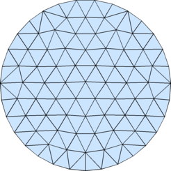
2D Implementation. The main goal of the Finite Elements Method is having a method able to work on a domain \(D\) no matter how complicated is its shape, bypassing the Finite Difference limitation to rectangular grids. This is accomplished mainly with the following two points: -
Generating a suitable mesh (possibly tailored on the specifics of the PDE) of \(D\) with \(N\) nodes \(\{p_1,\dots,p_N\}\) and a corresponding set of functions \(\{\psi_1,\dots,\psi_N\}\) such that:
- \(\psi_i(p_j)=\delta_{i,j}\,\text{;}\)
- \(\psi_i(p_i)=0\) on every mesh polygon not containing \(p_i\text{;}\)
- \(\psi_i\) has an absolute max at \(p_i\) and no other local max or saddle point on the polygons on which is not zero.
Using the PDE's weak version and restricting the eq. to \(\hbox{span}\,\{\psi_1,\dots,\psi_N\}\subset H^1(D)\text{.}\)
- The union \(M_D\) of all \(P_i\)'s is an approximation of \(D\text{,}\) namely the measure of the set of points not in \(M_D\cap D\) is small with respect to the measure of \(D\text{.}\)
- For any \(i\neq j\text{,}\) \(P_i\) and \(P_j\) are either disjoint or share a whole side; in particular, no vertex of one polygon falls in the interior of the side of another one.

m = 10;
n = 10;
[x,y] = ndgrid((0:m-1)/(m-1),(0:n-1)/(n-1));
pts = [x(:),y(:)];
tri = [1,2,m+2; 1,m+2,m+1];
tri = kron(tri,ones(m-1,1))+kron(ones(size(tri)),(0:m-2)');
tri = kron(tri,ones(n-1,1))+kron(ones(size(tri)),(0:n-2)'*m);
trimesh(tri,pts(:,1),pts(:,2))
A great starting point for generating 2D and 3D meshes with any sort off shape is Persson's Distmesh package. Functions Bases. We consider just the simplest type of mesh, where all polygons in a it are triangles. In this type of mesh, a reasonable set of \(\psi_i\) is the set of piece-wise linear functions that, on any triangle \(T\) of the mesh, are either identically zero or linear. Let \((x_i,y_i)\text{,}\) \(i=1,2,3\) be the vertices of \(T\) and \(\psi_i=a_i+b_ix+c_iy\text{,}\) \(i=1,2,3\text{,}\) the restriction to \(T\) of the three basis functions that are not identically zero on \(T\) and such that \(\psi_i(x_j,y_j)=\delta_{ij}\text{.}\) Then let
\begin{equation*}
M_T=
\begin{pmatrix}
1&x_1&y_1\cr
1&x_2&y_2\cr
1&x_3&y_3\cr
\end{pmatrix}\text{.}
\end{equation*}
The coefficients are solutions of
\begin{equation*}
M_T
\begin{pmatrix}
a_1\cr
b_1\cr
c_1\cr
\end{pmatrix}
=
\begin{pmatrix}
1\cr
0\cr
0\cr
\end{pmatrix}
,
\;
M_T
\begin{pmatrix}
a_2\cr
b_2\cr
c_2\cr
\end{pmatrix}
=
\begin{pmatrix}
0\cr
1\cr
0\cr
\end{pmatrix}
,
\;
M_T
\begin{pmatrix}
a_3\cr
b_3\cr
c_3\cr
\end{pmatrix}
=
\begin{pmatrix}
0\cr
0\cr
1\cr
\end{pmatrix}
,
\end{equation*}
namely
\begin{equation*}
\begin{pmatrix}
a_1&a_2&a_3\cr
b_1&b_2&b_3\cr
c_1&c_2&c_3\cr
\end{pmatrix}
=
M^{-1}_T
\end{equation*}
As in the previous case, the advantage of this choice is that the scalar products \(\langle\psi_i,\psi_j\rangle\) and \(\langle\psi'_i,\psi'_j\rangle\) are zero for \(|i-j|>1\text{,}\) so that the matrix \(A\) is tridiagonal.
Code 1. The MATLAB code below, by Niall Madden, is one of the most elementary implementation of the Finite Elements Method. It solves the Elliptic PDE
\begin{equation*}
\Delta u = 32(x(1-x)+y(1-y))
\end{equation*}
on the square \(S=[0,1]^2\) with Dirichlet boundary conditions \(u_{\partial S}=0\text{,}\) whose exact solution is
\begin{equation*}
u(x,y)=16xy(1-x)(1-y).
\end{equation*}
Code 2. Below I slightly modified the code above to make it work with Persson's DistMesh library and use it to solve the Poisson PDE
\begin{equation*}
\Delta u = 4(4x^2+4y^2-5)
\end{equation*}
on the annulus \(A=\{1\leq x^2+y^2\leq 4\}\) with Dirichlet boundary conditions \(u_{\partial A}=0\text{,}\) whose exact solution is
\begin{equation*}
u(x,y)=(4-x^2+y^2)(x^2+y^2-1).
\end{equation*}
Note that this code won't run on the web because the DistMesh library is not included in the standard Octave installation. In order to run it you need to cut&paste the code in your Octave or MATLAB folder, put in the same directory the DistMesh files and finally run the code. 