Section 2.5 Finite Differences Method: Elliptic PDEs
The most elementary Elliptic PDE,
\begin{equation*}
u_{xx} + u_{yy} = \rho\;\;\hbox{ in }S\,,\;\;u|_{\partial S}=f,
\end{equation*}
is named Poisson Equation or, when \(f=0\text{,}\) Laplace Equation.
Example: electrostatic electric potential. In case of static electric fields, the two Maxwell's laws
\begin{equation*}
{\mathbf\nabla}\cdot\mathbf E = \frac{\rho}{\varepsilon}
\,,\;\;
{\mathbf\nabla}\times\mathbf E = -\frac{\partial\mathbf B}{\partial t}\,,
\end{equation*}
amount to
\begin{equation*}
\mathbf E=-{\mathbf\nabla} V
\,,\;\;
\Delta V=-\frac{\rho}{\varepsilon}\,,
\end{equation*}
where \(V\) is the electric potential function associated to the (conservative) electric vector field \(\mathbf E\text{.}\)
Electric Potential of a point-like charge. Below we explore numerically the potential generated by a point charge \(q=4\pi\varepsilon\text{,}\) namely
\begin{equation*}
\Delta V(x,y) = 4\pi\delta(x-0.5,y-0.5)
\end{equation*}
for all \((x,y)\) in \(S=[0,1]\times[0,1]\text{.}\) Usually the potential \(V\) is set to zero at infinity and the solution is the well known potential of a charged point-like particle:
\begin{equation*}
V = \frac{1}{r}.
\end{equation*}
Below we will simply set \(V=0\) on the boundary of \(S\text{.}\)
Finite Differences - Explicit method. We replace the pts of \(S\) with the lattice \(\{i\Delta x,j\Delta y\}, 1\leq i,j\leq N\text{,}\) and
\begin{equation*}
V_{xx}(x_i,y_j)\to\frac{V_{i+1,j}-2V_{i,j}+V_{i-1,j}}{\left(\Delta x\right)^2}\text{,}
\end{equation*}
\begin{equation*}
V_{yy}(x_i,y_j)\to\frac{V_{i,j+1}-2V_{i,j}+V_{i,j-1}}{\left(\Delta y\right)^2}\text{,}
\end{equation*}
so that the equation translates into
\begin{equation*}
\frac{V_{i+1,j}-2V_{i,j}+V_{i-1,j}}{\left(\Delta x\right)^2}
+
\frac{V_{i,j+1}-2V_{i,j}+V_{i,j-1}}{\left(\Delta y\right)^2}
=
4\pi\rho_{i,j}
\;,\;\;
1\leq i,j\leq N
\end{equation*}
where \(\rho_{i,j}\) is equal to 1 at \((N/2,N/2)\) and zero everywhere else. We set \(\Delta x=\Delta y=h\text{,}\) so we get the following system:
\begin{equation*}
V_{i+1,j}+V_{i,j+1}-4V_{i,j}+V_{i-1,j}+V_{i,j-1}=4\pi h^2\rho_{i,j}
\end{equation*}
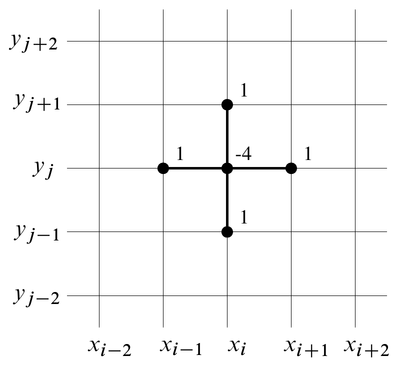
This Finite Differences scheme can be summarized by the 5-points stencil diagram below: 
\begin{equation*}
M = \begin{pmatrix}
B&-I&&&&&0\\
-I& B&-I&&&&\\
&.&.&.&&&\\
&&.&.&.&&\\
&&&.&.&.&\\
&&&&-I&B&-I\\
0&&&&&-I&B\\
\end{pmatrix}
\end{equation*}
is a \(N^2\) block matrix, where \(I\) is the \(N\times N\) identity matrix and
\begin{equation*}
B = \begin{pmatrix}
4&-1&&&&&0\\
-1& 4&-1&&&&\\
&.&.&.&&&\\
&&.&.&.&&\\
&&&.&.&.&\\
&&&&-1&4&-1\\
0&&&&&-1&4\\
\end{pmatrix}
\end{equation*}
Local Truncation Error. Let \(u(x,y)\) be the exact solution of the Poisson equation \(\Delta u=f\) and denote by \(\mathbf U\) the vector of all \(u(x_i,y_j)\) in lexicographic order. The vector \(\;\;\mathbf\tau = M\mathbf U-\mathbf R\;\;\text{,}\) whose components are
\begin{equation*}
\tau_{i,j}=\frac{u(x_{i-1},y_j)+u(x_{i+1},y_j)+u(x_{i},y_{j-1})+u(x_{i},y_{j+1})-4u(x_i,y_j)}{h^2}-f(x_i,y_j)\,,
\end{equation*}
represents the local truncation error for the 5-points stencil method. Via Taylor expansion we see that
\begin{equation*}
\tau_{i,j}=\frac{h^2}{12}\left[u_{xxxx}(x_i,y_j)+u_{yyyy}(x_i,y_j)\right]+O(h^4)
\end{equation*}
Global Error. Let \(\mathbf u = \hat u_{i,j}\) be the solution of the system \(M\mathbf u=\mathbf R\text{.}\) Then
\begin{equation*}
\mathbf E= \mathbf U-\mathbf u
\end{equation*}
is the global error of the method. This vector satisfies the equation
\begin{equation*}
M\mathbf E = M\mathbf U-M\mathbf u = \mathbf\tau +\mathbf R - \mathbf R = \mathbf\tau\,,
\end{equation*}
namely
\begin{equation*}
\mathbf E = M^{-1}\mathbf\tau\,.
\end{equation*}
Stability and Accuracy. Recall that the numerical solution of the Poisson equation through this method is
\begin{equation*}
\mathbf u = M^{-1}\mathbf R
\end{equation*}
and that \(\mathbf R\) is determined by the boundary conditions. In particular, the method is stable if the norm of the inverse stays bounded for \(h\to0\text{.}\) As a byproduct, if a method is stable then the global error is of the same order as the local one. Remark: all norms are equivalent in finite dimension, so this fact can be verified in the most convenient one. In this case it is convenient using the spectral norm. Since \(M\) is symmetric, its spectral norm is just its largest eigenvalue in modulus and the norm of \(M^{-1}\) is the inverse of the smallest eigenvalue in modulus of \(M\text{.}\) Hence it is enough to show that the spectrum of \(M\) stays far from the origin as \(h\to0\text{.}\) A direct calculation shows that the eigenvectors of \(M\) are the \(u_{i,j}^{p.q} = \sin(p\pi i h)\sin(q\pi jh),\;\;\;\;p,q=1,\dots,m\) with eigenvalues \(\lambda_{p,q} = \frac{2}{h^2}\left[\cos(p\pi h)-1+\cos(q\pi h)-1\right].\) The smallest in modulus of these eigenvalues is \(\lambda_{1,1} = \frac{2}{h^2}\left[\cos(\pi h)-1+\cos(\pi h)-1\right] \simeq -2\pi^2 + O(h^2),\) so that
\begin{equation*}
\|M^{-1}\|_{sp} = \frac{1}{-2\pi^2 + O(h^2)} = -\frac{1}{2\pi^2} + O(h^2),
\end{equation*}
namely \(M^{-1}\) is bounded in some nbhd of \(h=0\text{.}\)
Evaluating in concrete a numerical solution. We showed above that the 5-points stencil method has local and global order \(4\) in \(\Delta x=\Delta y=h\text{.}\) Finding the actual numerical solution to the Poisson equation \(\Delta u=f\) amounts to solving the linear system
\begin{equation*}
M\mathbf u=\mathbf R\,.
\end{equation*}
At this point, the PDE problem has become a linear algebra numerical problem. Methods to solve numerically linear systems can be found in any numerical anaysis introductory textbook. You can find a short introduction to this topic in these slides. Below we briefly discuss a few of these methods.
Solving \(M{\mathbf v}=\mathbf R\) - LU method. Write \(M=LU\text{,}\) with \(L\) lower and \(U\) upper triangular. \(LU{\mathbf v}=\mathbf R\) can be easily solved by forward and backward substitutions. The complexity of this method is \(O\left(N^3\right)\text{.}\) For banded matrices of bandwidth \(d\text{,}\) the complexity goes down to \(O\left(d^2N\right)\text{.}\)
Solving \(M{\mathbf v}=\mathbf R\) - Jacobi method Write \(M=L+D+U\text{,}\) with \(D\) diagonal, \(U\) upper and \(L\) lower diagonal. The solution is obtained iteratively by
\begin{equation*}
{\mathbf v}_{k+1} = -D^{-1}(L+U){\mathbf v}_{k} + D^{-1}\mathbf R
\end{equation*}
This converges to the solution iff the spectral radius of \(D^{-1}(L+U)\) is smaller than 1. This happens, for example, for diagonally dominant matrices. First Implementation in Python
Second Implementation in Python
Solving \(M{\mathbf v}=\mathbf R\) - Gauss-Seidel method Write \(M=L+D+U\text{,}\) with \(D\) diagonal, \(U\) upper and \(L\) lower diagonal. The solution is obtained iteratively by
\begin{equation*}
{\mathbf v}_{k+1} = -(L+D)^{-1}U{\mathbf v}_{k} + (L+D)^{-1}\mathbf R
\end{equation*}
The GS method converges when \(M\) is symmetric or diagonally dominant. For tridiagonal matrices, it is equivalent to Jacobi.
Solving \(M{\mathbf v}=\mathbf R\) - GS with SOR relaxation Write \(M=L+D+U\text{,}\) with \(D\) diagonal, \(U\) upper and \(L\) lower diagonal. The solution is obtained iteratively by
\begin{equation*}
{\mathbf v}_{k+1} = -(D+\omega L)^{-1}((1-\omega)D-\omega U){\mathbf v}_{k} + (D+\omega L)^{-1}\mathbf R
\end{equation*}
where \(0 < \omega < 2\)(it is sufficient for the convergence that \(A\) is symmetric and positive-definite). In general, the optimal \(\omega\) depends on the boundary conditions.