Section 1.7 Higher Order Methods: Multistep
The last way we illustrate to produce higher-order ODEs solvers is the one where one, in order to evaluate \((t_{n+1},x_{n+1})\text{,}\) rather than using just the slope \(f(t,x(t))\) at the previous point \((t_{n},x_{n})\text{,}\) uses the slopes previous \(k+1\) points
\begin{equation*}
(t_{n},f_{n}),\,(t_{n-1},f_{n-1}),\dots,\,(t_{n-k},f_{n-k}),
\end{equation*}
where we used the notation, that we will keep using throughout this section,
\begin{equation*}
f_i = f(t_i,x_i).
\end{equation*}
Just as in the Runge-Kutta case, this method uses the integral version of the IVP
\begin{equation*}
\dot x = f(t,x),\;x(t_0)=x_0
\end{equation*}
namely
\begin{equation*}
x_{n+1} = x_n + \int_{t_n}^{t_{n+1}} f(t,x(t))dt.
\end{equation*}
In this case, though, rather than subdiving the interval \([t_n,t_{n+1}]\) into \(k\) subintervals, as it is done in the Runge-Kutta case, it is the previous \(k\) steps of the algorithm that are used to evaluate the integral at the right hand side. Hence, in the \((k+1)\)-multistep method, in order to evaluate \((t_{n+1},x_{n+1})\text{,}\) the unknown function \(f(t,x(t))\text{,}\) where \(x(t)\) is the solution of the IVP above, is approximated by the unique polynomial \(p(t)\) whose value at the previous \((k+1)\) points found by the algorithm is exactly the value of \(f\) at those points.
Seeds. Since at each step are used the previous \(k+1\) values, we need to find somehow the first \(k+1\) points of the numerical solution. This can be obtained by using one of the single-step methods illustrated so far.
Euler. Notice that, for \(k=0\text{,}\) we get exactly the Euler method.
A crash-course in polynomial interpolation. There are two main methods to find the polynomial passing through \(k+1\) points \((t_{0},f_{0}),\dots,\,(t_{k},f_{k}).\) One is using Lagrange Polynomials. In short, define the \(k+1\) degree-\(k\) polynomials
\begin{equation*}
L_i(t) = \prod_{j\neq i}\frac{t-t_j}{t_i-t_j},\;i=0,\dots,k.
\end{equation*}
Then the sought polynomial is
\begin{equation*}
p(t) = \sum_{i=0}^k f_i L_i(t).
\end{equation*}
The second is using backward differences
\begin{equation*}
\nabla^0f_n=f_n,\;\nabla^{j+1}f_n=\nabla^j f_n-\nabla^jf_{n=1}.
\end{equation*}
According to Newton's interpolation formula,
\begin{equation*}
p(t) = \sum_{j=0}^k(-1)^j{-s\choose j}\nabla^j f_n,
\end{equation*}
where \(s=(t-t_n)/h\text{,}\) so that
\begin{equation*}
x_{n+1} = x_n + h\sum_{j=0}^k\gamma_j\nabla^jf_n.
\end{equation*}
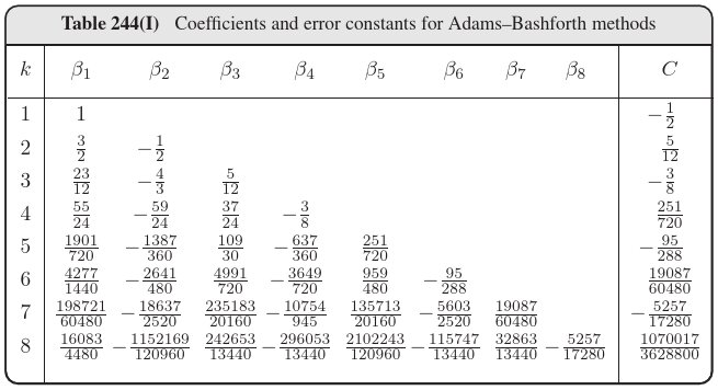
The following table (from Hairer, Norsett, Wanner, Solving ODEs I), shows the values of the first of these coefficients:

\begin{equation*}
x_{n+1} = \sum_{i=0}^{k}\beta_i f(t_{n-i},x_{n-i})
\end{equation*}
whose local error is given by
\begin{equation*}
C h^{k+1} x^{(k+1)}(\tau).
\end{equation*}
These algorithms are known as Adams-Bashforth methods. The values of the coefficients \(\beta_i\) and \(C\) are given in the table below (pls substract 1 from the value of \(k\) in the table below until I find the time to replace it).

\begin{equation*}
\begin{aligned}
&k=0:\;\;\;x_{n+1}=x_n+hf(t_n,x_n)\;\;\text{ (Euler method)}\\
&k=1:\;\;\;x_{n+1}=x_n+\frac{h}{2}\left(3f(t_n,x_n)-f(t_{n-1},x_{n-1})\right)\\
&k=2:\;\;\;x_{n+1}=x_n+\frac{h}{12}\left(23f(t_n,x_n)-16f(t_{n-1},x_{n-1})+5f(t_{n-2},x_{n-2})\right)\\
\end{aligned}
\end{equation*}
The case \(k=1\). Let us see in detail the case \(k=1\) using the Lagrange polynomials. The two points we will use to interpolate \(f(t,x(t))\) are \((t_n,f_n)\) and \((t_{n-1},f_{n-1})\text{.}\) The corresponding Lagrange polynomials are
\begin{gather*}
L_0(t) = \frac{t-t_{n-1}}{t_n-t_{n-1}}=\frac{1}{h}(t-t_{n}+h),\\
L_1(t) = \frac{t-t_{n}}{t_{n-1}-t_{n}}=-\frac{1}{h}(t-t_n)
\end{gather*}
and so the interpolating polynomial is
\begin{equation*}
p(t) = f_{n}L_0(t)+f_{n-1}L_1(t) = \frac{f_n}{h}(t-t_{n}+h) - \frac{f_{n-1}}{h}(t-t_n).
\end{equation*}
Hence the \(k=1\) Adams-Bashforth algorithm is
\begin{gather*}
x_{n+1} = x_n + \int_{t_{n}}^{t_n+h} p(t) = x_n + \frac{f_n}{2h}(t-t_{n}+h)^2\bigg|_{t_{n}}^{t_n+h} - \frac{f_{n-1}}{2h}(t-t_n)^2\bigg|_{t_{n}}^{t_n+h} =\\
= x_n + 2\frac{f_n}{h} - \frac{f_n}{2h} - \frac{f_{n-1}}{2h} = \\
= x_n + h\left(\frac{3}{2}f_n - \frac{1}{2}f_{n-1}\right).
\end{gather*}
Implementation of the case \(\mathbf{k=1}\). Below we solve our usual IVP
\begin{equation*}
\dot x=-x\cos t,\;\;x(0)=1
\end{equation*}
with the method with \(k=1\text{.}\)
Global error. By running the code above with different values of \(h\text{,}\) one can verify easily that the global order of this method is 2.
