AATA Riemann sums

Section 8.1 Riemann sums

The Fundamental Theorem of Calculus tells us that

$\begin{equation*} \int_a^bf(x)dx=F(b)-F(a) \end{equation*}$

for any antiderivative

$F(x)$ of

$f(x)\text{.}$ Unfortunately, though, very few functions have an antiderivative that can be written in terms of elementary functions. For instance,

$f(x)=e^{-x^2}$ does not!

🔗

The idea of numerical integration is to devise algorithms able to evaluate directly the integral as the area under the graph.

🔗

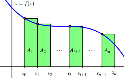
A simple example: Riemann sums. Every student already met such a method in Calculus 1: Riemann sums! For every continuous function (and many others), the Riemann integral can be defined as the limit of the left Riemann sum:

$\begin{equation*} \int_a^bf(x)dx=\lim_{n\to\infty}\left[f(a)+f(a+h)+\dots+f(a+(n-1)h)\right]h, \end{equation*}$

where

$h=(b-a)/n\text{.}$

🔗

Given some

$n\text{,}$ we can therefore approximate

$\int_a^b f(x)dx$ with

$\begin{equation*} L_n=\left[f(a)+f(a+h)+\dots+f(a+(n-1)h)\right]h. \end{equation*}$

Below is a simple MATLAB implementation of this algorithm, used to evaluate the integral of

$\sin x$ from 0 to 2.

xxxxxxxxxx
 
format long
a=0; b=2; h=0.01;
x=a:h:b;
x(end)=[]; %let's get rid of b
L = sum(h*sin(x)) % Riemann sum
I = 1-cos(2) % Exact value of the integral

🔗

Riemann sums error. How can we estimate the error we are making as function of

$n\text{?}$

🔗

Within each interval

$[a+kh,a+(k+1)h]\text{,}$ the worst that can happen is that

$f$ changes with constant rate of change equal to the maximum value of the derivative in that interval. In fact, to keep formulae simpler, we take the max of

$f'(x)$ over the whole interval

$[a,b]\text{.}$

🔗

We assume that

$f(x)$ has continuous first derivative, so that we are granted that

$M=\max_{[a,b]}|f'(x)|$ exists. Hence, the largest difference between the value of

$f(x)$ at

$a+kh$ and the one at

$a+(k+1)h$ is

$Mh\text{.}$

🔗

In turn, since the length of

$[a+kh,a+(k+1)h]$ is

$h\text{,}$ the highest possible error in the estimate of the integral in that interval is the area

$\frac{1}{2}Mh^2$ of the triangle with base

$h$ and height

$Mh\text{.}$

🔗

Since we have

$n=\frac{b-a}{h}$ summands, a bound to the total error is

$\begin{equation*} \left|\int_a^bf(x)dx-L_n\right|\leq\frac{b-a}{2}h\max_{[a,b]}|f'(x)|. \end{equation*}$

Convergence Speed. The formula above shows that the truncation error of the Riemann sum is

$O(h^1)\text{.}$ Below we visualize this scaling law by evaluating the error in the computation of

$\int_0^2\sin(x)dx\text{.}$

🔗

In this case, due to the slow convergence of this method, it is not possible to set

$h$ smaller than

$10^{-8}$ since otherwise the number of summands becomes too large to handle for either MATLAB or Octave. The minimum error achievable with this method for this integral is hence of the order of

$10^{-8}\text{.}$ Notice also that, in this range for

$h\text{,}$ the round-off component of the error is not visible.

xxxxxxxxxx
 
format long
n=8;
a=0; b=2; h(1)=0.1;
s = zeros(n); err = zeros(n);
for i = 1:n
    x=a:h(i):b; % these are the x_i
    x(end)=[]; %let's get rid of b
    s(i)=sum(h(i)*sin(x)); % this is the integral
    err(i)=abs(1-cos(2)-s(i)); % and this is the actual error
    h(i+1) = h(i)/10; 
end
x=2:n;
clf
[h(x)' err(x)']
loglog(h(x),err(x));
hold on
loglog(h(x),h(x));
xlabel('h') 
ylabel('y') 
legend({'y=error(h)','y=h'},'Location','northwest')