
Section 6.1 What does it mean optimizing a function
Optimizing a function of \(n\) variables \(f:\Bbb R^n\to\Bbb R\) means finding its extrema, namely its local maxima and minima. Since a max of \(f(\boldsymbol{x})\) is a min for \(g(\boldsymbol{x})=-f(\boldsymbol{x})\text{,}\) we will consider just the case of the search for local minima. Critical Points. Recall that the critical points (also called extrema) of a function \(f(\boldsymbol{x})\) with continuous first derivative are all zeros of the gradient
\begin{equation*}
\nabla f(\boldsymbol{x}) = \left(f_{x_1}(\boldsymbol{x}),f_{x_2}(\boldsymbol{x}),\dots,f_{x_n}(\boldsymbol{x})\right).
\end{equation*}
which is a vector with \(n\) components. Its zeros are therefore the solutions of a system of \(n\) equations in \(n\) variables.
Remark 6.1.1.
Here and throughout the book, we use the notation \(f_x\) to denote the partial derivative of \(f\) with respect the variable \(x\text{,}\) since the notation \(\partial f/\partial x\) would take too much space.
\begin{equation*}
Hess(f) =
\begin{pmatrix}
f_{x^1x^1}&f_{x^1x^2}&\dots&f_{x^1x^n}\\
f_{x^2x^1}&f_{x^2x^2}&\dots&f_{x^2x^n}\\
\vdots&\ddots&\ddots&\vdots\\
f_{x^nx^1}&f_{x^nx^2}&\dots&f_{x^nx^n}\\
\end{pmatrix}
\end{equation*}
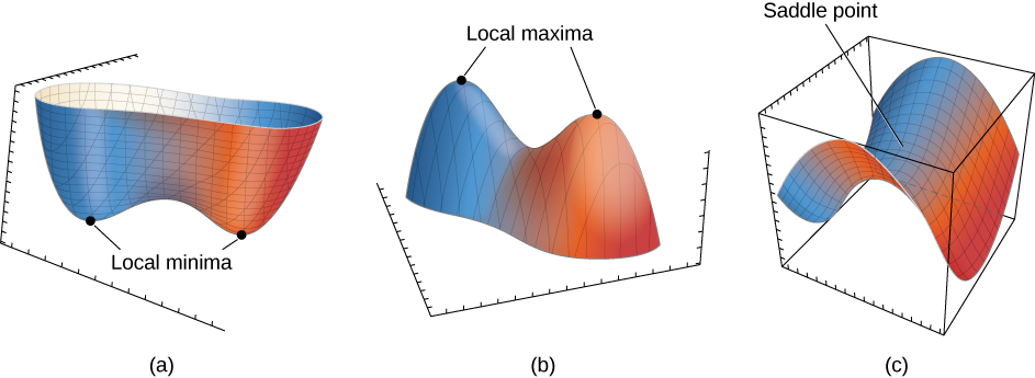
at the point \(\boldsymbol{x_0}\text{.}\) Recall that mixed partial derivatives commute with each other and so the Hessian matrix is always symmetric. As we recalled in the previous chapter, symmetrix matrices have always all real eigenvalues. What dictates the type of a critical point is exactly the spectrum of the Hessian: - if all eigenvalues of \(Hess_{\boldsymbol{x_0}}(f)\) are positive (i.e. \(Hess_{\boldsymbol{x_0}}(f)\) is positive-definite), then \(\boldsymbol{x_0}\) is a local minimum;
- if all eigenvalues of \(Hess_{\boldsymbol{x_0}}(f)\) are negative (i.e. \(Hess_{\boldsymbol{x_0}}(f)\) is negative-definite), then \(\boldsymbol{x_0}\) is a local maximum;
- otherwise, \(\boldsymbol{x_0}\) is a saddle.
\begin{equation*}
f(x) = \frac{1}{2}\boldsymbol{x}^TA\boldsymbol{x} - b^T\boldsymbol{x} +c
\end{equation*}
where \(A\) is a \(n\times n\) symmetric matrix, \(b\) a vector with \(n\) components and c a number. A direct calculation shows that
\begin{equation*}
Hess(f) = A,
\end{equation*}
namely in this case the Hessian is constant (just like the second derivative of a quadratic function in one variable). Then, \(f(x)\) has a minimum if and only f all eigenvalues of \(A\) are positive. Since
\begin{equation*}
\nabla f(x) = A\boldsymbol{x} - b,
\end{equation*}
the position of the minimum coincides with the solution of the linear system
\begin{equation*}
A\boldsymbol{x}=b.
\end{equation*}
Equivalence of Optimization and Root-finding. Since critical points are solutions of \(n\times n\) systems, every optimization problem is a root-finding problem and so it can be solve by any root-finding method (see Chapter 3). The inverse is also true. Given any function of \(n\) variables \(f(x)\text{,}\) each of its zeros is a clearly minimum for the function \(F(x) = \left(f(x)\right)^2\text{,}\) since the square of a real number cannot be negative. Hence, all optimization methods can be used to find roots.