
Section 6.6 Conjugate Gradient
A shortcoming of the steepest descent method to solve \(Ax=b\) is that it tends to "zig-zag" a lot, namely we come back often to the same (or almost the same) direction many times when, close to the minimum, the level sets are ellipses with high eccentricity -- see the picture below.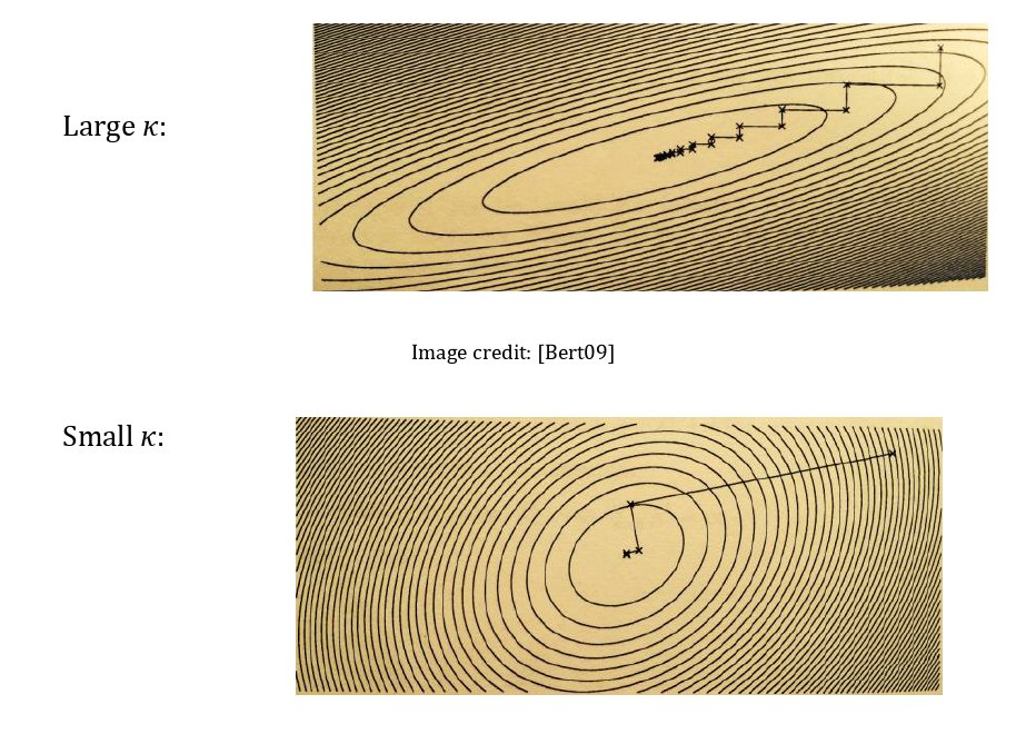
Definition 6.6.1.
A scalar product \(\langle,\rangle\) on a vector space \(V\) is a map associating to a pair of vectors a real number so that:- \(\langle u,v \rangle = \langle v,u \rangle\) (symmetry)
- \(\langle \lambda u+\mu v,w \rangle = \lambda \langle u,w \rangle + \mu \langle v,w \rangle\) (linearity)
- \(\langle v,v \rangle > 0\) for \(v\neq0\) (positivity)
\begin{equation*}
\|v\|^2 = \langle v,v \rangle
\end{equation*}
but the inverse is not true (will show this below). What is relevant for us is that every scalar product, in coordinates, is represented by a quadratic polynomial. Indeed, take any basis \(\{e_1,\dots,e_n\}\) of \(V\text{,}\) so that
\begin{equation*}
v=\sum_{i=1}^n v_i e_i\;\hbox{ and }\;u=\sum_{i=1}^n u_i e_i.
\end{equation*}
Then, because of the linearity,
\begin{equation*}
\langle u,v \rangle = \left\langle \sum_{i=1}^n u_i e_i,\sum_{j=1}^n v_j e_j \right \rangle = \sum_{i,j=1}^n u_iv_j \langle e_i,e_j \rangle = \sum_{i,j=1}^n u_iv_j G_{ij} = u^T\cdot G\cdot v.
\end{equation*}
This is precisely a quadratic homogeneous polynomial in the components of \(v\) and \(u\text{.}\) The last expression is a re-writing of the double summation as a matricial product -- it will be useful to write scalar products in Python.
Eigenvalues of the matrix \(G\). How do reflect on \(G\) the symmetry and positivity of the scalar product \(\langle , \rangle\text{?}\) - \(G\) must be symmetric (just choose \(u=e_i\) and \(v=e_j\) and apply the symmetry). In particular, this means that the eigenvalues of \(G\) are all real and that there is some basis of \(V\) where \(G\) writes as a diagonal matrix.
- The eigenvalues of \(G\) are all positive (easy to prove in a basis of eigenvectors).
\begin{equation*}
f(x)=\frac{1}{2}x^TAx-\boldsymbol{b}^Tx+c.
\end{equation*}
We can always consider the matrix \(A\) symmetric because it appears in a symmetric expression. Then, by Theorem 6.4.3, we know that \(f\) has a minimum if and only if \(A\) has all eigenvalues strictly positive. Hence, the expression
\begin{equation*}
\langle u,v \rangle_A = u^T\cdot A\cdot u
\end{equation*}
is a scalar product. Notice also that, viceversa, given any scalar product \(\langle , \rangle\text{,}\) the function
\begin{equation*}
f(x) = \langle x,x \rangle
\end{equation*}
is quadratic in \(x\text{.}\)
The idea behind the algorithm. We finally have enough ingredients to come up with a nice algorithm to fuind the minimum of
\begin{equation*}
f(x)=\frac{1}{2}x^TAx-\boldsymbol{b}^Tx+c.
\end{equation*}
Recall first of all that
\begin{equation*}
\nabla_x f = Ax-b
\end{equation*}
and so the location of the minimum of \(f\) is the solution of the linear system
\begin{equation*}
Ax=b.
\end{equation*}
Denote by \(x_*\) that solution -- notice that there is a unique solution because \(A\) has, by hypothesis, all strictly positive eigenvalues and so it is invertible -- and denote by \(\{\epsilon_1,\dots,\epsilon_n\}\) any basis of \(V\) that is orthogonal with respect to the scalar product \(\langle , \rangle_A\) induced by \(A\text{,}\) namely assume that
\begin{equation*}
\epsilon_i^T\cdot A\cdot \epsilon_j = 0\;\hbox{ for }\;i\neq j.
\end{equation*}
Then
\begin{equation*}
x_* = \sum_{i=1}^n \alpha_i \epsilon_i
\end{equation*}
and
\begin{equation*}
\epsilon_i^T\cdot b = \epsilon_i^T\cdot A\cdot x_* = \epsilon_i^T\cdot A\sum_{j=1}^n \alpha_j \epsilon_j = \sum_{i=1}^n \alpha_j \epsilon_i^T\cdot A\cdot \epsilon_j = \sum_{i=1}^n \alpha_j\langle \epsilon_i,\epsilon_j \rangle_A = \alpha_i.
\end{equation*}
This gives us an algorithm to get to \(x_*=A^{-1}b\) in at most \(n\) steps: - start at \(x_0=0\text{;}\)
- for \(i=1,\dots,n\text{,}\) move by \(\epsilon_i^T\cdot b\) times the vector \(\epsilon_i\text{.}\)
\begin{equation*}
\epsilon_1 = -\nabla_{x_0} f = b-Ax_0.
\end{equation*}
Then we move by \(\alpha_1 \epsilon_1\) and, at the arrival point, we look for the vector \(\epsilon_1\)\(A\)-orthogonal to \(\epsilon_1\) and contained in the plane spanned by \(\nabla_{x_0} f\) and \(\nabla_{x_1} f\text{,}\) namely
\begin{equation*}
\epsilon_2 = -\nabla_{x_1} f + \frac{\epsilon_1^T\cdot A\cdot \nabla_{x_0}f}{\epsilon_1^TA\epsilon_1}\epsilon_1
\end{equation*}
and so on. Ultimately, we end up with the following algorithm:
\begin{equation*}
\begin{aligned}
\alpha_k&=\frac{\|\boldsymbol{r}_{k}\|^2}{\|\boldsymbol{p}_{k}\|^2_A}=\frac{\boldsymbol{r}^T_{k}\boldsymbol{r}_{k}}{\boldsymbol{p}^T_{k}A\boldsymbol{p}_{k}}\\
\boldsymbol{x}_{k+1}&=\boldsymbol{x}_{k} + \alpha_k\boldsymbol{p}_{k}\\
\boldsymbol{r}_{k+1}&=\boldsymbol{b}-A\boldsymbol{x}_{k}=\boldsymbol{r}_{k}-\alpha_kA\boldsymbol{p}_{k} \\
\beta_k&=\frac{\langle \boldsymbol{r}_{k+1},\boldsymbol{p}_{k}\rangle_A}{\|\boldsymbol{p}_{k}\|^2}
=\frac{\|\boldsymbol{r}_{k+1}\|^2}{\|\boldsymbol{r}_{k}\|^2}\\
\boldsymbol{p}_{k+1}&=\boldsymbol{r}_{k+1}+\beta_k\boldsymbol{p}_{k}\\
\end{aligned}
\end{equation*}
Code 1. Below we find the minimum of our usual quadratic function
\begin{equation*}
f(x,y)=5x^2+4xy+y^2-6x-4y+15
\end{equation*}
with this method. In this first implementation, we use the very same matricial notation used above.
Code 2. The code below minimize the same quadratic function using a more general notation: - At each step
k, the variableris defined as the opposite of the gradient at the current pointx[:,k]. - Similarly, the matrix
Ais defined as the Hessian matrix at the current pointx[:,k](notice that in this case, since the function is quadratic, the Hessian is constant).
\begin{equation*}
g(x,y)=f(x,y)+2x^4+x^2y^2.
\end{equation*}
(by Ben Frederikson).