NA Shooting Method

🔗

Section 9.10 Shooting Method

🔗

Assuming that there is a solution to

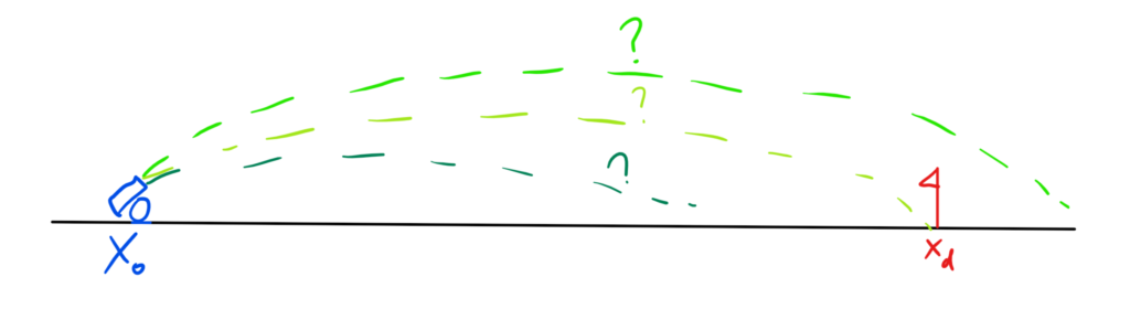
$\begin{equation*} \ddot x=f(t,x,\dot x)\,,\;x(t_0)=x_0\,,\;x(t_f)=x_f\,, \end{equation*}$

the shooting method's idea is using IVP to find better and better approximations of the value of

$\dot x(t_0)$ that produces a solution

$x(t)$ s.t.

$x(t_f)=x_f\text{.}$

🔗

Clearly indeed by assigning values

$v$ to

$\dot x(t_0)$ we obtain a function

$F(v)$ defined as the value of

$x(t_f)$ when

$\dot x(t_0)=v\text{.}$ The shooting method consists exaclty in applying some numerical method, such as the Newton method, to solve the equation

$F(v)=x_f\text{,}$ namely to find the initial value of

$\dot x(t)$ such that the point arrives at

$x_f$ at

$t=t_f\text{.}$

🔗

Subsection 9.10.1 The Linear Case

A particularly simple case it the linear one. Recall the following theorem:

🔗

Theorem 9.10.1.

The space of solutions of a linear ODE

$\begin{equation*} \dot x = Ax,\,x(t_0)=x_0,\,x\in\Bbb R^n \end{equation*}$

is itself a linear space. Moreover, the map that sends an initial condition

$x_0$ to the corresponding solution is a linear map.

🔗

In fact, the explicit expression of that map is given by

$\begin{equation*} x_0\mapsto x(t) = e^{A(t-t_0)}x_0. \end{equation*}$

In particular, this means that for linear BVP

$\begin{equation*} \ddot x = a(t) \dot x + b(t) x +c(t),\,x(t_0) = x_0,\, x(t_f)=x_f, \end{equation*}$

the function

$F(v)$ is itself linear, namely

$\begin{equation*} F(v) = \alpha v+\beta. \end{equation*}$

Hence it is enough to solve numerically two IVP in order to solve the BVP. For instance, say that

$F(0) = q_0$ and

$F(1) = q_1\text{.}$ Then

$\beta = q_0$ and

$\alpha = q_1-q_0\text{,}$ so that the solution to

$\begin{equation*} F(v) = x_f \;\;\mbox{ is }\;\; v = \frac{x_f-q_0}{q_1-q_0}. \end{equation*}$

Example. Consider the IVP

$\begin{equation*} \dot x = -x\cos t,\,x(0)=1,\, \end{equation*}$

whose solution is

$x(t)=e^{-\sin t}\text{.}$

🔗

Since we need a 2nd order ODE,

🔗

we will rather consider the BVP given by its "first prolongation"

$\begin{equation*} \ddot x = -\dot x\cos t+x\sin t,\,x(0)=1,\,x(15\pi/2)=e. \end{equation*}$

The code below applies the method illustrade above to solve this BVP.

xxxxxxxxxx
 
from numpy import linspace, zeros, cos, sin, pi
import matplotlib.pyplot as plt
​
N = 100; ti = 0.; tf = 15*pi/2; xi = 1; xf = exp(1); h = tf/N;
​
#Solving a first time the ODE with explicit Euler's method...
q0=xi; p0=0; T=linspace(ti,tf,N+1)
for i in range(N):
    a = q0
    q0 = q0 + h*p0
    p0 = p0 + h*(-p0*cos(T[i])+a*sin(T[i]))
​
qf0 = q0
pf0 = p0
​
#Solving a second time the ODE with explicit Euler's method...
q1=xi
p1=1
for i in range(N):
    a = q1
    q1 = q1 + h*p1
    p1 = p1 + h*(-p1*cos(T[i])+a*sin(T[i]))
​
qf1 = q1
pf1 = p1
​
#Solving last time the ODE with explicit Euler's method...
Q = zeros(N+1)
P = zeros(N+1)
Q[0]=xi
P[0]=(xf-qf0)/(qf1-qf0)
for i in range(N):
   Q[i+1] = Q[i] + h*P[i];
   P[i+1] = P[i] + h*(-P[i]*cos(T[i])+Q[i]*sin(T[i]));
​
exactSolution = lambda t: exp(-sin(t))
​
plt.clf()
plt.plot(T,Q,'ro-',T,exactSolution(T),'b-');
plt.legend(["Numerical solution, h = {}".format(h),"Exact solution"])
plt.show()