Analytic semigroup are a special breed of semigroups, as they allow for more regularity of the solutions. The Laplacian will, in many situations, lead to an analytic semigroup, hence it is of relevance in many applications. We have made use of complex analysis occasionally within this book. Now it is time to dig in even deeper.
Proposition9.11.1.
Let \(f(z)\) be an analytic function in a domain \(D(f)\subset \CC\) and \(\gamma\subset D(f)\) a closed positively oriented curve (i.e., oriented counterclockwise). Then
It turns out that analytic semigroup can be characterized by the spectrum of the generator.
Definition9.11.2.
Let \((A,D(A))\) be a closed linear operator on a Banach space \(X\text{.}\) A is called sectorial if there exists an angle \(0<\delta<\frac{\pi}{2}\) such that the sector
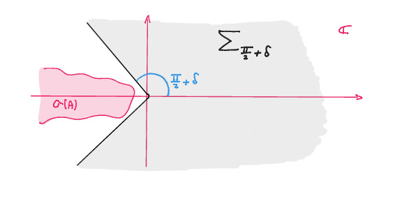
In Figure 9.11.3 we illustrate the spectrum of \(A\) and the sector \(\Sigma_{\frac{\pi}{2}+\delta}\) which is spanned by the angles \(\frac{\pi}{2}+\delta\) and \(-\frac{\pi}{2} - \delta\text{,}\) excluding the origin.
Figure9.11.3.Schematic showing the sector $\Sigma_{\frac{\pi The estimate above is a uniform resolvent estimate on a sector that is slightly smaller than \(\Sigma_{\frac{\pi}{2}+\delta}\text{.}\) The constant \(M_\ep\) will grow as we get closer and closer to the boundary of \(\Sigma_{\frac{\pi}{2}+\delta}\text{,}\) i.e. as \(\ep\to 0\text{,}\) and it can not be expected that \(M_\ep\) stays bounded as we reach the boundary of \(\Sigma_{\frac{\pi}{2}+\delta}\text{.}\) See Figure [cross-reference to target(s) "f-page17" missing or not unique].
Figure9.11.4.Uniform resolvent estimates in a slightly smaller sector $\Sigma_{\frac{x We use the Cauchy Integral Formula to represent the semigroup.
Definition9.11.5.
Let \((A,D(A))\) be densely defined and sectorial with angle \(\delta\text{.}\) We define an operator family \(\{T(z)\}\) with complex argument \(z\) as \(T(0)=I\) and for \(z\in \Sigma_\delta\)
for some \(\delta'\in (|\mbox{arg } z|, \delta). \) Notice the level of strangeness in this definition. Remember that for a semigroup, we were looking at an operator family that depends on a scalar variable \(t\text{,}\) which is often understood as time. In this context, the semigroup property is a very natural assumption, which says that a system evolving to \(t+s\) must first evolve to \(t\) and then \(s\) units more. So what does it mean for \(T\) to depend on a complex variable \(z\text{?}\) Is this a complex time? Well, of course not, but the positive real axis is a part of the complex plane, and for a real world application we can simply restrict \(T(z)\) to \(T(t)\) and keep our physical meaning. In addition we find that close to the real axis, we can extend the semigroup to a semigroup with complex arguments. \\ Notice that \(T(z)\) in (Definition 9.11.5) is defined on a much much smaller sector \(\Sigma_\delta\) than the sector we considered earlier \(\Sigma_{\frac{\pi}{2}+\delta}\text{.}\) As we show in Figure [cross-reference to target(s) "f-page18" missing or not unique] for small \(\delta\) the sector \(\Sigma_\delta\text{,}\) is just a small stripe above and below the positive real axis.
Figure9.11.6.The semigroup \(T(z)\) is defined in a small sector \(\Sigma_\delta\) around the positive \(x\)-axis.
Theorem9.11.7.
Let \((A,D(A))\) be a densely defined sectorial operator with angle \(\delta\text{.}\) Then for all \(z\in \Sigma_\delta\) the maps \(T(z)\) are bounded linear operators on \(X\) with the following properties
\(\|T(z)\|\) is uniformly bounded in each smaller sector \(\Sigma_{\delta'}\text{,}\) \(0<\delta'<\delta\text{.}\)
The map \(z\mapsto T(z)\) is analytic in \(\Sigma_\delta\text{,}\) i.e. we call \(\{T(z)\}\) and analytic semigroup.
For all \(z_1, z_2 \in \Sigma_\delta\) with \(z_1+z_2\in \Sigma_\delta\) we have
\(\ep=\frac{1}{2}(\delta -\delta'). \)[cross-reference to target(s) "f-page19" missing or not unique]
Figure9.11.8.The construction of the path \(\gamma_r\) and the sector \(\Sigma_\delta\) as used in the proof.\(z\in \Sigma_{\delta'}\)\(r=\frac{1}{|z|}\text{.}\)\(\mu\in \gamma_{r,3}\)\(z\in \Sigma_{\delta'}\)
To show strong continuity, we consider the map \(z\mapsto T(z)\) and show continuity at \(z=0\text{.}\) The semigroup property item 3. does the rest. We come back to the path \(\gamma_r\) defined earlier, but now we chose specific radius \(r=1\text{,}\) i.e. the path \(\gamma_1\text{.}\) Note that \(0\) is inside this path, hence we have
Now, in (Definition 9.11.5), we define a semigroup through a complex path integral. Are these definitions the same, at least for real arguments \(T(t)\text{?}\) The answer is the next theorem.
Theorem9.11.10.
Let \(\{T(z)\}\) be the analytical semigroup defined by (Definition 9.11.5). Then the sectorial operator \((A,D(A))\) is its generator.
Let \(\{T(z)\}\) be defined through (Definition 9.11.5) and denote by \((B, D(B))\) the generator of \(\{T(t)\}\text{.}\) We show that \(R_\lambda(B) = R_\lambda(A)\) for a very particular \(\lambda\in \rho(A)\text{.}\) Because if \(R_\lambda(A)=R_\lambda(B)\text{,}\) then \((A-\lambda I)=(B-\lambda I)\) and \(A=B\text{.}\) Set \(\lambda = |\omega|+2\text{,}\) where \(\omega\) is the growth rate of \(T(t)\text{,}\) and use the Laplace transform formula for the resolvent
\begin{equation*}
R_\lambda(B) x = -\int_0^\infty e^{-\lambda t} T(t) x dt.
\end{equation*}
We again employ the specific path \(\gamma_1\) with radius \(r=1\) near zero. Then
\begin{align*}
-\int_0^{t_0} e^{-\lambda t} T(t) x \, dt \amp=\amp \frac{-i}{2\pi} \int_0^{t_0} \ointop_{\gamma_1} e^{-\lambda t}e^{\mu t} R_\mu(A) x \, d\mu\, dt\\
\amp=\amp \frac{1}{2\pi i} \ointop_{\gamma_1} \frac{e^{t_0(\mu-\lambda)} -1}{\mu-\lambda} R_\mu(A) x d\mu.
\end{align*}
We close \(\gamma_1\) as shown in Figure [cross-reference to target(s) "f-page22" missing or not unique]. Now, \(\gamma_1\) is clockwise, hence we get a minus sign. Also, \(\gamma_1\) encloses the point \(\lambda=|\omega|+2\text{.}\) Hence we get
\begin{equation}
-\int_0^{t_0} e^{-\lambda t} T(t) x \, dt =
R_\lambda(A) x +\frac{1}{2\pi i} \ointop_{\gamma_1} \frac{e^{t_0(\mu-\lambda)}}{\mu-\lambda} R_\mu(A) d\mu. \tag{9.11.3}
\end{equation}
Since \(\lambda=|\omega|+2,\) we have \(\lambda>2\text{,}\) and on \(\gamma_1\) we have \(\max\{\mbox{Re}(\mu)\} =1\text{,}\) which implies \(\mbox{Re}(\lambda-\mu) \geq 1\text{.}\) Hence \(e^{t_0(\mu-\lambda)} \leq e^{-t_0}\text{.}\) And since \(|\lambda-\mu|>|\mu|\text{,}\) the under-braced integral is bounded by \(\int_1^\infty \frac{M_\ep}{\mu^2} d\mu\text{,}\) which is bounded. Hence for \(t_0\to\infty\text{,}\) we get indeed
\begin{equation*}
R_\lambda(B) x = R_\lambda(A) x,
\end{equation*}
for all \(x\in X\text{.}\)
Figure9.11.11.The construction of the path \(\gamma_1\) for the proof of Theorem Theorem 9.11.10
\((A,D(A))\) is densely defined and sectorial for any angle \(0<\delta<\frac{\pi}{2}.\) Hence \(T(t)= \exp(t \frac{d^2}{dx^2}) \) is a analytic semigroup in a sector \(\Sigma_\delta\) around the positive real axis.
And the reverse of Theorem Theorem 9.11.10 is true as well, which we cite without proof. A proof, which is quite a bit more involved, can be found in the book of Engel and Nagel \cite{Engel} Theorem 4.6, p 95.
Theorem9.11.13.
If \(A\) generates an analytic semigroup \(\{T(z)\}\) then \(A\) is sectorial.
Remark9.11.14.
We now complete our Semigroup Triangle. In Figure [cross-reference to target(s) "semigrouptriangle3" missing or not unique]. We fill in all connections that we identified. Note that the connection between the resolvent \(R_\lambda\) and the semigroup \(T\) via the Cauchy integral formula is only valid for analytic semigroups. \tikzstyle{semigr} = [ellipse, draw, fill=red!30, text width=3cm, text centered, minimum height=4em] \tikzstyle{gener} = [ellipse, draw, fill=yellow!40, text width=3cm, text centered, minimum height=4em] \tikzstyle{resol} = [ellipse, draw, fill=blue!20, text width=3cm, text centered, minimum height=4em] \tikzstyle{arrow} =[thick,->, >=stealth]